Regularization L-curves

This tutorial demonstrates how to do a regularization L-curve, using the Spherical Integral Geometric Tensor Tomography (SIGTT) pipeline as a guiding example, since it has a built-in regularizer.

The dataset of trabecular bone used in this tutorial is available via Zenodo, and can be downloaded either via a browser or the command line using, e.g., wget or curl,

wget https://zenodo.org/records/10074598/files/trabecular_bone_9.h5

import warnings
from mumott.data_handling import DataContainer
from mumott.pipelines import run_sigtt
import matplotlib.pyplot as plt
import colorcet
import logging
import numpy as np
data_container = DataContainer('trabecular_bone_9.h5')

INFO:Setting the number of threads to 4. If your physical cores are fewer than this number, you may want to use numba.set_num_threads(n), and os.environ["OPENBLAS_NUM_THREADS"] = f"{n}" to set the number of threads to the number of physical cores n.
INFO:Setting numba log level to WARNING.
INFO:Inner axis found in dataset base directory. This will override the default.
INFO:Outer axis found in dataset base directory. This will override the default.
INFO:Rotation matrices were loaded from the input file.
INFO:Sample geometry loaded from file.
INFO:Detector geometry loaded from file.

SIGTT - Spherical Integral Geometric Tensor Tomgraphy

SIGTT is a relatively straightforward reconstruction method. The reciprocal space map at one q-bin is a function on the sphere, and therefore it can be expressed in spherical harmonics. They are orthogonal and rotationally invariant, and therefore converge easily. Correlation between neighbours can be easily expressed in terms of the spherical harmonic inner product, or power-spectrum function, and one can maximize this correlation by minimizing the Laplacian. This is the basic motivation behind the SIGTT pipeline.

The pipeline uses the LBFGS-B optimizer. We will first run the pipeline without any regularization by setting the weight to zero. We will use an ftol of 1e-4, maxiter of 50, and maxfun of np.inf, to discourage overly eager convergence.

%%time
result = run_sigtt(data_container,
                   use_gpu=True,
                   optimizer_kwargs=dict(ftol=1e-4, maxfun=np.inf, maxiter=50),
                   regularization_weight=0.)
reconstruction = result['result']['x']
output = result['basis_set'].get_output(reconstruction)

 50%|█████     | 25/50 [00:48<00:48,  1.96s/it]
CPU times: user 1min 30s, sys: 7.34 s, total: 1min 37s
Wall time: 49.4 s

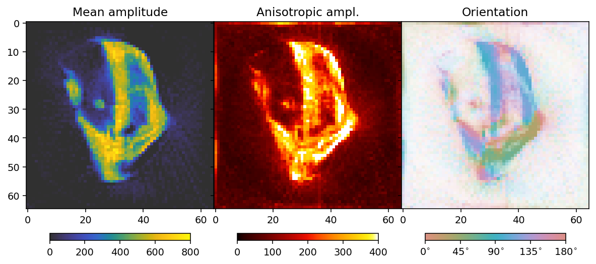
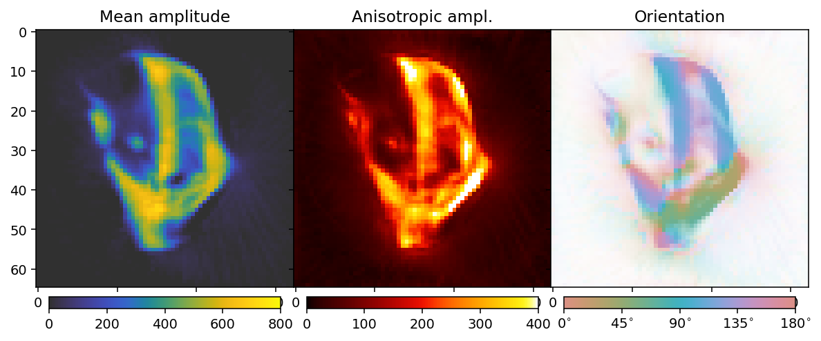
To analyze the results we here define a convenience function that allows us to extract mean, fractional anisotropy, and orientation data in a 2D slice from the reconstruction.

The function defined here uses output.eigenvector_1 which corresponds to the direction with lowest scattering, For equatorial ring type scattering output.eigenvector_1 is apropriate. For polar cap type scattering, output.eigenvector_3.

plotted_slice_index = 28
mask_threshold = 200

def get_2d_images(output):

    mean = output.mean_intensity[plotted_slice_index]
    mask = mean > mask_threshold

    fractional_anisotropy = output.fractional_anisotropy[plotted_slice_index]
    fractional_anisotropy[~mask] = 1

    main_eigenvector = output.eigenvector_1[plotted_slice_index]
    orientation = np.arctan2(-main_eigenvector[..., 1],
                             main_eigenvector[..., 2])
    orientation[orientation < 0] += np.pi
    orientation[orientation > np.pi] -= np.pi
    orientation *= 180 / np.pi

    alpha = np.clip(output.fractional_anisotropy[plotted_slice_index], 0, 1)
    alpha[~mask] = 0

    return mean, fractional_anisotropy, orientation, alpha

mean, fractional_anisotropy, orientation, alpha = get_2d_images(output)

Next we plot the results.

colorbar_kwargs = dict(orientation='horizontal', shrink=0.75, pad=0.1)
mean_kwargs = dict(vmin=0, vmax=800, cmap='cet_gouldian')
fractional_anisotropy_kwargs = dict(vmin=0, vmax=1.0, cmap='cet_fire')
orientation_kwargs = dict(vmin=0, vmax=180, cmap='cet_CET_C10')

def config_cbar(cbar):
    cbar.set_ticks([i for i in np.linspace(0, 180, 5)])
    cbar.set_ticklabels([r'$' + f'{int(v):d}' + r'^{\circ}$' for v in bar.get_ticks()])

fig, ax = plt.subplots(1, 3, figsize=(10.3, 4.6), dpi=140, sharey=True)

im0 = ax[0].imshow(mean, **mean_kwargs);
im1 = ax[1].imshow(fractional_anisotropy, **fractional_anisotropy_kwargs);
im2 = ax[2].imshow(orientation, alpha=alpha, **orientation_kwargs);

ax[0].set_title('Mean amplitude')
ax[1].set_title('Fractional anisotropy')
ax[2].set_title('Orientation')

plt.subplots_adjust(wspace=0)

plt.colorbar(im0, ax=ax[0], **colorbar_kwargs)
plt.colorbar(im1, ax=ax[1], **colorbar_kwargs)
bar = plt.colorbar(im2, ax=ax[2], **colorbar_kwargs)
config_cbar(bar)

First regularization weight sweep

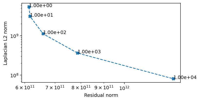
In order to find the optimal value for the regularization, we need to check a wide span, and investigate how the residual norm changes relative to the regularization norm.

%%time
weights = np.geomspace(1e-2, 1e5, 5)
results = []
residual_norm = []
regularization_norm = []
for i, w in enumerate(weights):
    results.append(run_sigtt(data_container,
                             use_gpu=True,
                             optimizer_kwargs=dict(ftol=1e-4, maxfun=np.inf, maxiter=50),
                             regularization_weight=w))
    residual_norm.append(results[i]['loss_function'].get_residual_norm()['residual_norm'])
    regularization_norm.append(results[i]['loss_function'].get_regularization_norm()['laplacian']['regularization_norm'])

 50%|█████     | 25/50 [00:45<00:45,  1.82s/it]
 56%|█████▌    | 28/50 [01:06<00:52,  2.38s/it]
 48%|████▊     | 24/50 [00:42<00:45,  1.77s/it]
 52%|█████▏    | 26/50 [00:42<00:39,  1.64s/it]
 18%|█▊        | 9/50 [00:18<01:24,  2.06s/it]
CPU times: user 6min 55s, sys: 35.4 s, total: 7min 31s
Wall time: 3min 36s

reconstructions = [r['result']['x'] for r in results]
outputs = [r['basis_set'].get_output(r['result']['x']) for r in results]

colorbar_kwargs = dict(orientation='horizontal', shrink=0.9, pad=0.03)
fig, axes = plt.subplots(ncols=3, nrows=5, figsize=(6.8, 12.8), dpi=140, sharey=True, sharex=True)
for i in range(5):
    ax = axes[i]
    mean, fractional_anisotropy, orientation, alpha = get_2d_images(outputs[i])
    plt.subplots_adjust(wspace=0, hspace=0)
    im0 = ax[0].imshow(mean, **mean_kwargs);
    im1 = ax[1].imshow(fractional_anisotropy, **fractional_anisotropy_kwargs);
    im2 = ax[2].imshow(orientation, alpha=alpha, **orientation_kwargs);
    if i == 0:
        ax[0].set_title('Mean amplitude')
        ax[1].set_title('Fractional anisotropy')
        ax[2].set_title('Orientation')
    ax[0].set_ylabel(r'$\lambda = ' + f'{weights[i]:.2e}' + r'$')
    if i == 4:
        plt.colorbar(im0, ax=axes[:, 0], **colorbar_kwargs);
        plt.colorbar(im1, ax=axes[:, 1], **colorbar_kwargs);
        bar = plt.colorbar(im2, ax=axes[:, 2], **colorbar_kwargs);
        config_cbar(bar)

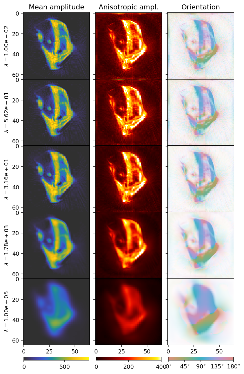
With increasing \(\lambda\), the reconstruction becomes blurrier. We can get a better idea by looking at the an L-curve.

f, ax = plt.subplots(1, 1, figsize=(6, 3), dpi=140)
ax.loglog(residual_norm, regularization_norm, '--X')
for x, y, t in zip(residual_norm, regularization_norm, weights):
    ax.text(x, y, f'{t:.2e}')
ax.set_ylabel('Laplacian L2 norm')
ax.set_xlabel('Residual norm')

Text(0.5, 0, 'Residual norm')

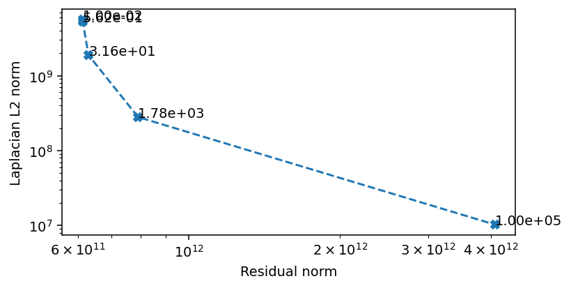
The critical area where the Laplacian L2 norm and the residual norm are simultaneously minimized is when the regularization weight is between \(1\) and \(1e4\). We scan this region in more detail to find a preferred value.

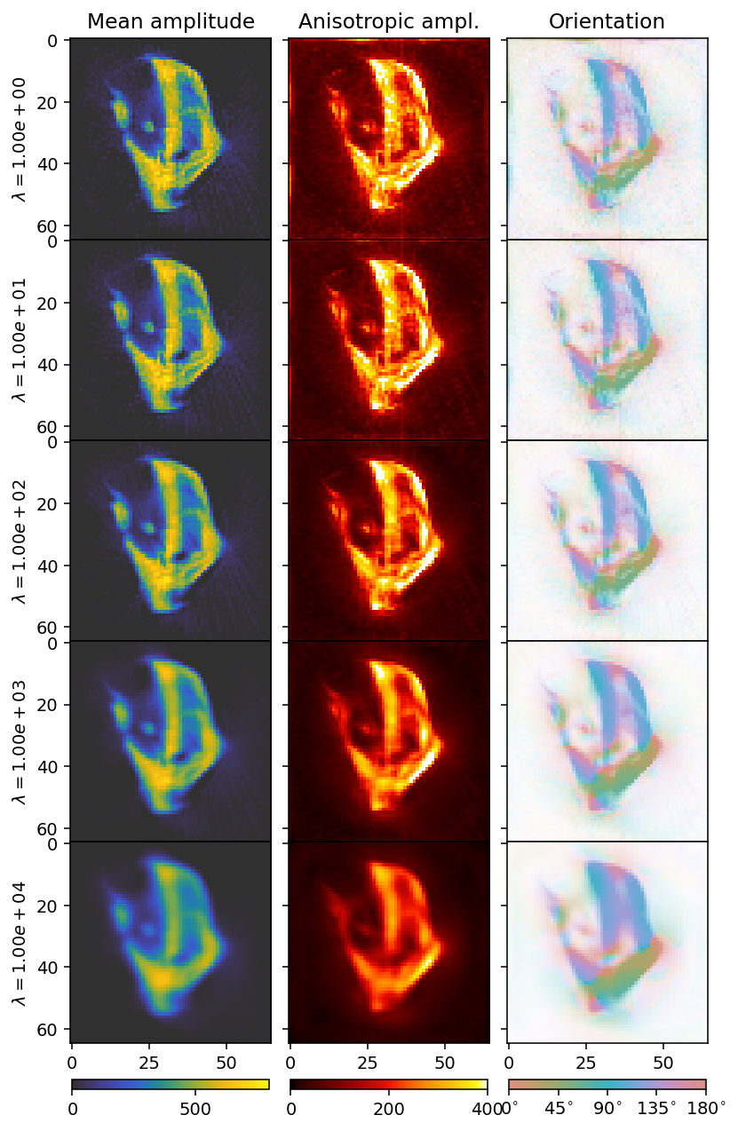
Second sweep

%%time
weights = np.geomspace(1, 1e4, 5)
results = []
residual_norm = []
regularization_norm = []
for i, w in enumerate(weights):
    results.append(run_sigtt(data_container,
                             use_gpu=True,
                             optimizer_kwargs=dict(ftol=1e-5, gtol=1e-7, maxfun=np.inf, maxiter=100),
                             regularization_weight=w))
    residual_norm.append(results[i]['loss_function'].get_residual_norm()['residual_norm'])
    regularization_norm.append(results[i]['loss_function'].get_regularization_norm()['laplacian']['regularization_norm'])

 25%|██▌       | 25/100 [00:45<02:17,  1.83s/it]
 25%|██▌       | 25/100 [00:42<02:08,  1.72s/it]
 23%|██▎       | 23/100 [00:41<02:20,  1.82s/it]
 22%|██▏       | 22/100 [00:54<03:13,  2.48s/it]
 27%|██▋       | 27/100 [00:36<01:39,  1.36s/it]
CPU times: user 7min 14s, sys: 33.7 s, total: 7min 48s
Wall time: 3min 43s

reconstructions = [r['result']['x'] for r in results]
outputs = [r['basis_set'].get_output(r['result']['x']) for r in results]

colorbar_kwargs = dict(orientation='horizontal', shrink=0.9, pad=0.03)
fig, axes = plt.subplots(ncols=3, nrows=5, figsize=(6.8, 12.8), dpi=140, sharey=True, sharex=True)
for i in range(5):
    ax = axes[i]
    mean, fractional_anisotropy, orientation, alpha = get_2d_images(outputs[i])
    plt.subplots_adjust(wspace=0, hspace=0)
    im0 = ax[0].imshow(mean, **mean_kwargs);
    im1 = ax[1].imshow(fractional_anisotropy, **fractional_anisotropy_kwargs);
    im2 = ax[2].imshow(orientation, alpha=alpha, **orientation_kwargs);
    if i == 0:
        ax[0].set_title('Mean amplitude')
        ax[1].set_title('Fractional anisotropy')
        ax[2].set_title('Orientation')
    ax[0].set_ylabel(r'$\lambda = ' + f'{weights[i]:.2e}' + r'$')
    if i == 4:
        plt.colorbar(im0, ax=axes[:, 0], **colorbar_kwargs);
        plt.colorbar(im1, ax=axes[:, 1], **colorbar_kwargs);
        bar = plt.colorbar(im2, ax=axes[:, 2], **colorbar_kwargs);
        config_cbar(bar)

f, ax = plt.subplots(1, 1, figsize=(6, 3), dpi=140)
ax.loglog(residual_norm, regularization_norm, '--X')
for x, y, t in zip(residual_norm, regularization_norm, weights):
    ax.text(x, y, f'{t:.2e}')
ax.set_ylabel('Laplacian L2 norm')
ax.set_xlabel('Residual norm')

Text(0.5, 0, 'Residual norm')

There seems to be three regions, which we can also infer from the convergence rate. At weights below \(1e1\) the convergence is dominated by the residual norm. Above \(1e3\) the convergence is dominated by the regularization. The area of interest ins the region in between, where we also see the most rapid convergence. We can conclude that a value in this range is likely to be optimal, and we opt for \(5e2\) as our weight.

The final result

%%time
result = run_sigtt(data_container,
                   use_gpu=True,
                   optimizer_kwargs=dict(ftol=1e-5, gtol=1e-7, maxfun=np.inf, maxiter=100),
                   regularization_weight=5e2,
                   maxiter=100)
reconstruction = result['result']['x']
output = result['basis_set'].get_output(reconstruction)

 17%|█▋        | 17/100 [00:32<02:41,  1.94s/it]
CPU times: user 1min 2s, sys: 5.32 s, total: 1min 7s
Wall time: 33.5 s

mean, fractional_anisotropy, orientation, alpha = get_2d_images(output)

fig, ax = plt.subplots(1, 3, figsize=(10.3, 4.6), dpi=140, sharey=True)

im0 = ax[0].imshow(mean, **mean_kwargs);
im1 = ax[1].imshow(fractional_anisotropy, **fractional_anisotropy_kwargs);
im2 = ax[2].imshow(orientation, alpha=alpha, **orientation_kwargs);

ax[0].set_title('Mean amplitude')
ax[1].set_title('Fractional anisotropy')
ax[2].set_title('Orientation')

plt.subplots_adjust(wspace=0)

plt.colorbar(im0, ax=ax[0], **colorbar_kwargs)
plt.colorbar(im1, ax=ax[1], **colorbar_kwargs)
bar = plt.colorbar(im2, ax=ax[2], **colorbar_kwargs)
config_cbar(bar)

This reconstruction has a reasonable tradeoff between blurring detail and reducing noise. The Laplacian has drawbacks as a regularizer, due to its tendency to blur edges, but regularizers which are more edge- and detail-preserving such as the \(L_1\) and Total Variation either risk inducing rotational biases, or are more difficult to obtain convergence and interpret L-curves for. Thus, while the Laplacian is not necessarily the best regularizer in practice, it is a good case study for learning the basics of regularization.