Aligning data
This tutorial demonstrates the alignment pipeline in mumott. We will use a publically available experimental data dataset of trabecular bone, for which the alignment has already been done. This allows us to demonstrate the procedure and compare our results to an independent reference.
Below we briefly inspect the original data. We then reset the alignment and apply the MITRA pipeline to reconstruct the data. If successful this should allow us to reproduce the quality of the original alignment.
The data set used in this tutorial is available via Zenodo, and can be downloaded either via a browser or the command line using, e.g., wget or curl,
wget https://zenodo.org/records/10074598/files/trabecular_bone_9.h5
[1]:
import logging
import numpy as np
import matplotlib.pyplot as plt
import colorcet
from ipywidgets import interact
from mumott.data_handling import DataContainer
from mumott.pipelines.utilities.alignment_geometry import shift_center_of_reconstruction
from mumott.pipelines import run_phase_matching_alignment as align
from mumott.pipelines import run_mitra

logger = logging.getLogger('mumott.optimization.optimizers.gradient_descent')
logger.setLevel(logging.WARNING)
INFO:Setting the number of threads to 8. If your physical cores are fewer than this number, you may want to use numba.set_num_threads(n), and os.environ["OPENBLAS_NUM_THREADS"] = f"{n}" to set the number of threads to the number of physical cores n.
INFO:Setting numba log level to WARNING.
Inspecting the original data
We begin by loading the data.
[2]:
dc = DataContainer('trabecular_bone_9.h5')
INFO:Inner axis found in dataset base directory. This will override the default.
INFO:Outer axis found in dataset base directory. This will override the default.
INFO:Rotation matrices were loaded from the input file.
INFO:Sample geometry loaded from file.
INFO:Detector geometry loaded from file.
The geometry is already aligned, so we will have a look at that alignment first.
[3]:
geo = dc.geometry
display(geo)
Geometry
| Field | Size | Data |
|---|---|---|
| rotations | 247 | 6ca379 (hash) |
| j_offsets | 247 | 14c068 (hash) |
| k_offsets | 247 | 794be2 (hash) |
| p_direction_0 | 3 | [0. 0. 1.] |
| j_direction_0 | 3 | [0. 1. 0.] |
| k_direction_0 | 3 | [1. 0. 0.] |
| inner_angles | 247 | b43664 (hash) |
| outer_angles | 247 | 3e8e01 (hash) |
| inner_axes | 247 | 5e6ea6 (hash) |
| outer_axes | 247 | 3da038 (hash) |
| detector_direction_origin | 3 | [1. 0. 0.] |
| detector_direction_positive_90 | 3 | [0. 1. 0.] |
| two_theta | 1 | [0.]${}^{\circ}$ |
| projection_shape | 2 | [65 55] |
| volume_shape | 3 | [55 65 65] |
| detector_angles | 8 | [0.2 ... 2.95] |
| full_circle_covered | 1 | False |
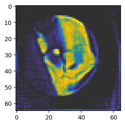
Let us run a reconstruction of the absorbance to see what to expect if the data is well aligned. We also save the projector object from for further use. It will be automatically updated with changes to the geometry.
[4]:
%%time
pipeline_reference = run_mitra(dc, use_gpu=True, maxiter=25)
reconstruction_reference = pipeline_reference['result']['x']
projector = pipeline_reference['projector']
projection_reference = projector.forward(reconstruction_reference)
100%|█| 25/25 [00:03<00:00,  7.72it/s]
CPU times: user 5.23 s, sys: 467 ms, total: 5.69 s
Wall time: 5.69 s
[5]:
fig, ax = plt.subplots(figsize=(3.2, 3.2), dpi=140)
ax.imshow(reconstruction_reference[28, :, :, 0], vmin=0, vmax=0.05, cmap='cet_gouldian');
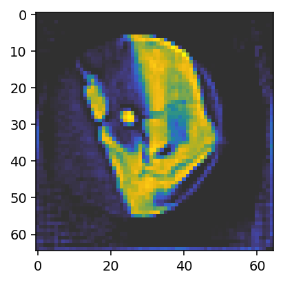
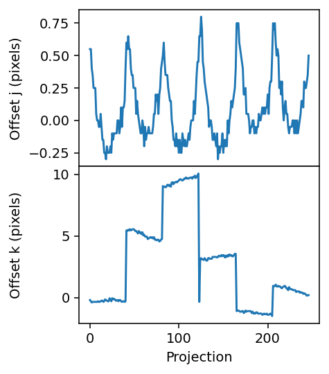
The reconstruction looks OK as expected for aligned data. We can also plot the alignments to get a sense for their distribution.
[6]:
fig, axes = plt.subplots(figsize=(3.2, 4.2), sharex=True, nrows=2, dpi=140)

axes[0].plot(geo.j_offsets)
axes[1].plot(geo.k_offsets)

axes[1].set_xlabel('Projection')
axes[0].set_ylabel('Offset j (pixels)')
axes[1].set_ylabel('Offset k (pixels)')

plt.subplots_adjust(hspace=0)
fig.align_ylabels()
We keep a copy of the alignment from the original dataset and reinitialize the offsets.
[7]:
j_offsets_reference = geo.j_offsets
k_offsets_reference = geo.k_offsets
geo.j_offsets = np.zeros(len(geo), dtype=np.float64)
geo.k_offsets = np.zeros(len(geo), dtype=np.float64)
At the end of this tutorial we want to visualize the effect of the alignment. Before we carry out the alignment procedure, we therefore run the reconstruction pipeline once and keep a copy of the result (reconstruction_run1).
[8]:
%%time
reconstruction_unaligned = run_mitra(dc, use_gpu=True, maxiter=25)['result']['x']
projections_unaligned = projector.forward(reconstruction_unaligned)
100%|█| 25/25 [00:03<00:00,  8.02it/s]
CPU times: user 6.76 s, sys: 415 ms, total: 7.17 s
Wall time: 7.17 s
First run
We now run the alignment.
We are going to pass a few keyword arguments:
maxiter– We start out with 30 iterations but expect the reconstruction to converge before the end.use_gpu– We use the GPU for calculating the projections and back-projections of the reconstruction. Set this argument toFalseif you do not have a GPU.projection_cropping- We crop the projection a bit to avoid fitting to edge artefacts.reconstruction_pipeline_kwargs– These are the keyword arguments passed to the reconstruction pipeline. We will use25iterations throughout. If the reconstruction runs slowly on your hardware, you might want to set this lower.use_gpuwill be passed along here.
[9]:
%%time
result = align(dc,
               use_gpu=True,
               maxiter=30,
               projection_cropping=np.s_[8:-8, 8:-8],
               reconstruction_pipeline_kwargs=dict(maxiter=25))
j_offsets_run1 = geo.j_offsets
k_offsets_run1 = geo.k_offsets
100%|█| 30/30 [02:29<00:00,  4.98s/it]
INFO:Maximal number of iterations reached. Alignment completed.
CPU times: user 2min 18s, sys: 11.2 s, total: 2min 29s
Wall time: 2min 29s
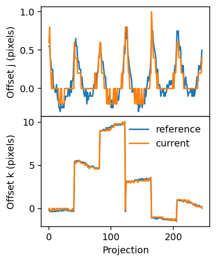
Let us inspect the result. We can use the reconstruction from the results, but it is better to rerun the same reconstruction pipeline that we originally used.
[10]:
%%time
reconstruction_run1 = run_mitra(dc, use_gpu=True, maxiter=25)['result']['x']
100%|█| 25/25 [00:03<00:00,  8.10it/s]
CPU times: user 3.58 s, sys: 361 ms, total: 3.94 s
Wall time: 3.93 s
[11]:
fig, ax = plt.subplots(figsize=(3.2, 3.2), dpi=140)
ax.imshow(reconstruction_run1[28, :, :, 0], vmin=0, vmax=0.05, cmap='cet_gouldian');
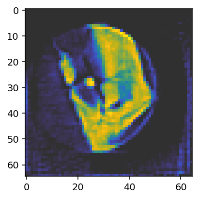
The result is not quite as good as the one obtained above using the reference alignment, but it is already reasonably close. Let us compare the alignments.
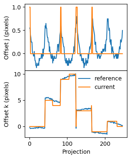
[12]:
fig, axes = plt.subplots(figsize=(3.2, 4.2), sharex=True, nrows=2, dpi=140)

axes[0].plot(j_offsets_reference)
axes[0].plot(geo.j_offsets)
axes[1].plot(k_offsets_reference, label='reference')
axes[1].plot(geo.k_offsets, label='current')

axes[1].set_xlabel('Projection')
axes[0].set_ylabel('Offset j (pixels)')
axes[1].set_ylabel('Offset k (pixels)')
axes[1].legend(frameon=False)

plt.subplots_adjust(hspace=0)
fig.align_ylabels()
Second run
One can observe in the results from the first tun that the offsets are overall reasonable in magnitude but limited to integer values. In the next step, we run the alignment procedure again but using a moderate upsampling factor (upsampling=5). This will allow for non-integer offsets, i.e., subpixel resolution.
[13]:
%%time
result = align(dc,
               use_gpu=True,
               upsampling=5,
               projection_cropping=np.s_[8:-8, 8:-8],
               reconstruction_pipeline_kwargs=dict(maxiter=25))
j_offsets_run2 = geo.j_offsets
k_offsets_run2 = geo.k_offsets
 35%|▋ | 7/20 [00:38<01:13,  5.64s/it]INFO:Maximal shift is 0.00, which is less than the specified tolerance 0.20. Alignment completed.
 35%|▋ | 7/20 [00:43<01:21,  6.25s/it]
CPU times: user 40.6 s, sys: 3.01 s, total: 43.6 s
Wall time: 43.8 s
Again, we re-run the original pipeline and compare.
[14]:
%%time
reconstruction_run2 = run_mitra(dc, use_gpu=True, maxiter=25)['result']['x']
100%|█| 25/25 [00:03<00:00,  8.04it/s]
CPU times: user 3.62 s, sys: 332 ms, total: 3.95 s
Wall time: 3.94 s
[15]:
fig, ax = plt.subplots(figsize=(3.2, 3.2), dpi=140)
ax.imshow(reconstruction_run2[28, :, :, 0], vmin=0, vmax=0.05, cmap='cet_gouldian');
[16]:
fig, axes = plt.subplots(figsize=(3.2, 4.2), sharex=True, nrows=2, dpi=140)

axes[0].plot(j_offsets_reference)
axes[0].plot(geo.j_offsets)
axes[1].plot(k_offsets_reference, label='reference')
axes[1].plot(geo.k_offsets, label='current')

axes[1].set_xlabel('Projection')
axes[0].set_ylabel('Offset j (pixels)')
axes[1].set_ylabel('Offset k (pixels)')
axes[1].legend(frameon=False)

plt.subplots_adjust(hspace=0)
fig.align_ylabels()
The result is even closer to the reference solution. One can also observe how the upsampling factor (5) determines the values that the offset can assume. This is especially apparent in the upper panel, where the curve shows steps of 0.2=1/5.
Third run
To finish, let us carry out a run with a larger upsampling factor (upsampling=20).
[17]:
%%time
result = align(dc,
               maxiter=30,
               use_gpu=True,
               upsampling=20,
               projection_cropping=np.s_[8:-8, 8:-8],
               reconstruction_pipeline_kwargs=dict(maxiter=25))
j_offsets_run3 = geo.j_offsets
k_offsets_run3 = geo.k_offsets
100%|█| 30/30 [02:44<00:00,  5.47s/it]
INFO:Maximal number of iterations reached. Alignment completed.
CPU times: user 2min 52s, sys: 1min 52s, total: 4min 44s
Wall time: 2min 44s
[18]:
%%time
pipeline_run3 = run_mitra(dc, use_gpu=True, maxiter=25)
reconstruction_run3 = pipeline_run3['result']['x']
projections_run3 = pipeline_run3['projector'].forward(reconstruction_run3)
100%|█| 25/25 [00:03<00:00,  7.89it/s]
CPU times: user 6.55 s, sys: 657 ms, total: 7.21 s
Wall time: 6.87 s
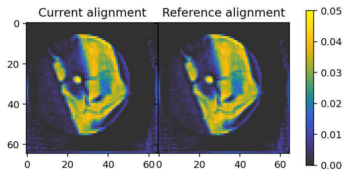
[19]:
fig, axes = plt.subplots(figsize=(6, 3), ncols=2, dpi=140, sharex=True, sharey=True)
kwargs = dict(vmin=0, vmax=0.05, cmap='cet_gouldian')

im_1 = axes[0].imshow(reconstruction_run3[28, :, :, 0], **kwargs);
im_2 = axes[1].imshow(reconstruction_reference[28, :, :, 0], **kwargs);
axes[0].set_title('Current alignment')
axes[1].set_title('Reference alignment')

plt.subplots_adjust(wspace=0)
plt.colorbar(im_2, ax=axes, shrink=0.95);
[20]:
fig, axes = plt.subplots(figsize=(3.2, 4.2), sharex=True, nrows=2, dpi=140)

axes[0].plot(j_offsets_reference)
axes[0].plot(j_offsets_run3, '--')
axes[1].plot(k_offsets_reference, label='reference')
axes[1].plot(k_offsets_run3, '--', label='current')

axes[1].set_xlabel('Projection')
axes[0].set_ylabel('Offset j (pixels)')
axes[1].set_ylabel('Offset k (pixels)')
axes[1].legend(frameon=False)

plt.tight_layout()
plt.subplots_adjust(hspace=0)
fig.align_ylabels()
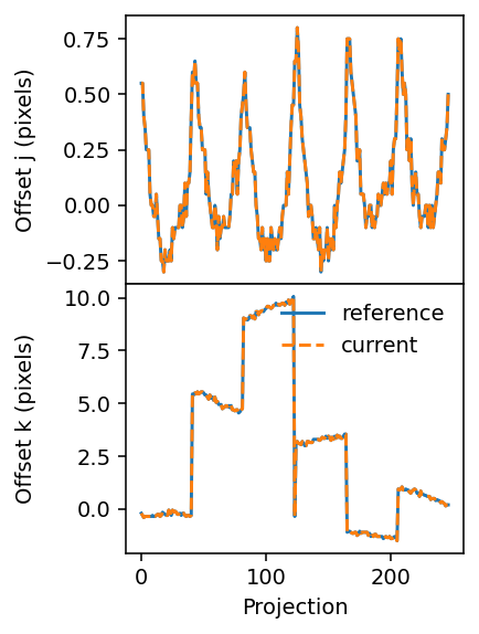
We have now obtained alignment offsets that appear identical to the ones originally in the data.
Comparing projections
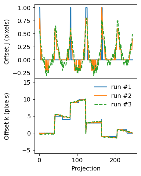
To wrap up, let us first inspect the progression of the offsets during the three runs.
[21]:
fig, axes = plt.subplots(figsize=(3.2, 4.2), sharex=True, nrows=2, dpi=140)

ax = axes[0]
ax.plot(j_offsets_run1)
ax.plot(j_offsets_run2)
ax.plot(j_offsets_run3, '--')
ax.set_ylabel('Offset j (pixels)')

ax = axes[1]
ax.plot(k_offsets_run1, label='run #1')
ax.plot(k_offsets_run2, label='run #2')
ax.plot(k_offsets_run3, '--', label='run #3')
ax.set_xlabel('Projection')
ax.set_ylabel('Offset k (pixels)')
ax.legend(frameon=False)
ax.set_ylim(-6, 16)

plt.tight_layout()
plt.subplots_adjust(hspace=0)
fig.align_ylabels()
Finally, we check the projections against the computed absorbances used to align them. To do this effectively one can use the interactive %matplotlib widget setting, which can be activated by removing the comment sign (#) on the first line of the following cell. (For the purpose of rendering this tutorial in HTML it has been commented out here.)
[22]:
#%matplotlib widget

fig, axes = plt.subplots(figsize=(12, 3), ncols=4, dpi=140, sharex=True, sharey=True)

kwargs = dict(vmin=0, vmax=1, cmap='cet_gouldian')
im_0 = axes[0].imshow(projections_unaligned[0, ..., 0], **kwargs)
im_1 = axes[1].imshow(projections_run3[0, ..., 0], **kwargs)
im_2 = axes[2].imshow(projection_reference[0, ..., 0], **kwargs)
im_3 = axes[3].imshow(result['reference'][0, ..., 0], **kwargs)

axes[0].set_title('Without alignment')
axes[1].set_title('Current alignment')
axes[2].set_title('Reference alignment')
axes[3].set_title('Data')

plt.subplots_adjust(wspace=0)
plt.colorbar(im_2, ax=axes, shrink=0.95)

@interact(i=(0, len(dc.geometry) - 1, 1))
def update(i=128):
    if i < 0 or i >= len(dc.geometry):
        return
    im_0.set_data(projections_unaligned[i, ..., 0])
    im_1.set_data(projections_run3[i, ..., 0])
    im_2.set_data(projection_reference[i, ..., 0])
    im_3.set_data(result['reference'][i, ..., 0])
    im_0.set_clim(-0.1, 1.1)
    im_1.set_clim(*im_0.get_clim())
    im_2.set_clim(*im_0.get_clim())
    im_3.set_clim(*im_0.get_clim())
    fig.canvas.flush_events()
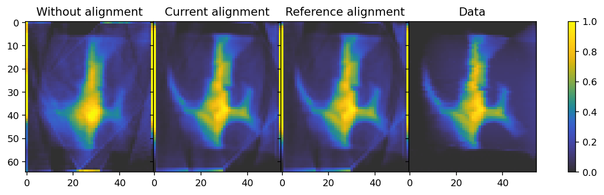
We can see some streaks in certain reconstructed projections, such as projection 0, regardless of alignment. This likely results from the fact that the sample is embedded in a substrate, part of which moves in and out of view at certain orientations. Regardless, the resulting alignment is very simimlar to both the reference alignment, as well as to the data, and a very large improvement over the unaligned reconstruction.
Saving
Finally, we can save our alignment results to file. This allows us to reload the alignment information later and apply it during a full reconstruction.
[23]:
geo.write('alignment.geo')