Reconstruction and visualization¶

This is a brief tutorial that demonstrates how to do a basic reconstruction and visualization of a data set in 2D and 3D, and explains some of the parameters necessary for the reconstruction to work correctly. The reconstruction only requires the usage of CPU resources. The simulated data used in the rendered version of this tutorial can be obtained using, e.g., wget with

wget https://zenodo.org/records/7326784/files/saxstt_dataset_M.h5

[1]:

import h5py
import matplotlib.pyplot as plt
import numpy as np
from IPython.display import display
from ipywidgets import interact
from mumott.data_handling import DataContainer
from mumott.output_handling import ProjectionViewer
from mumott.output_handling.saving import dict_to_h5
from mumott.methods.basis_sets import SphericalHarmonics
from mumott.methods.projectors import SAXSProjector
from mumott.methods.residual_calculators import GradientResidualCalculator
from mumott.optimization.loss_functions import SquaredLoss
from mumott.optimization.optimizers import LBFGS
from mumott.optimization.regularizers import Laplacian

INFO:Setting the number of threads to 8
INFO:Setting numba log level to WARNING.

Loading data¶

First, we need to locate our input data. The path, name, and input type are defined as strings. The path can be either relative or absolute. The file name needs to include the file ending. The only allowed input format is 'h5' (which requires a specially formated hdf5 file).

Initializing the DataContainer¶

The input files must contain most of the necessary metadata, so creating a DataContainer object simply requires passing the file name as an argument.

[2]:

data_container = DataContainer('saxstt_dataset_M.h5')

INFO:Rotation matrix generated from inner and outer angles, along with inner and outer rotation axis vectors. Rotation and tilt angles assumed to be in radians.

mumott/data_handling/data_container.py:227: DeprecationWarning: Entry name rotations is deprecated. Use inner_angle instead.
  _deprecated_key_warning('rotations')
mumott/data_handling/data_container.py:236: DeprecationWarning: Entry name tilts is deprecated. Use outer_angle instead.
  _deprecated_key_warning('tilts')
mumott/data_handling/data_container.py:268: DeprecationWarning: Entry name offset_j is deprecated. Use j_offset instead.
  _deprecated_key_warning('offset_j')
mumott/data_handling/data_container.py:278: DeprecationWarning: Entry name offset_k is deprecated. Use k_offset instead.
  _deprecated_key_warning('offset_k')

INFO:No sample geometry information was found. Default mumott geometry assumed.
INFO:No detector geometry information was found. Default mumott geometry assumed.

We can now take a quick look at the container object to see that the parameters make sense.

[3]:

display(data_container)

DataContainer

Field	Size
Number of projections	417
Corrected for transmission	False

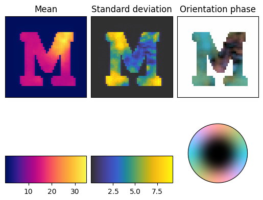
We can use the ProjectionViewer to check out projections. For interactive usage, it would be necessary to use the setting %matplotlib widget, but for the purpose of correctly rendering the widget in HMTL, this is left out.

[4]:

p = ProjectionViewer(data_container, orientation_symmetry='transversal')

@interact(i=(0, len(data_container), 1))
def change_projection(i=0):
    p.change_projection(i)

mumott/output_handling/orientation_image_mapper.py:22: MatplotlibDeprecationWarning: The get_cmap function was deprecated in Matplotlib 3.7 and will be removed two minor releases later. Use ``matplotlib.colormaps[name]`` or ``matplotlib.colormaps.get_cmap(obj)`` instead.
  self._colormap = get_cmap(colormap)
mumott/output_handling/projection_viewer.py:137: MatplotlibDeprecationWarning: The get_cmap function was deprecated in Matplotlib 3.7 and will be removed two minor releases later. Use ``matplotlib.colormaps[name]`` or ``matplotlib.colormaps.get_cmap(obj)`` instead.
  self._phase_colormap_lut = cm.get_cmap(self._phase_colormap, 256)
colorspacious/ciecam02.py:333: RuntimeWarning: invalid value encountered in divide
  t = (C
ipywidgets/widgets/interaction.py:43: DeprecationWarning: `ipykernel.pylab.backend_inline` is deprecated, directly use `matplotlib_inline.backend_inline`
  from ipykernel.pylab.backend_inline import flush_figures

../_images/tutorials_reconstruct_and_visualize_8_1.png

We now need to choose a basis set (we choose SphericalHarmonics with ell_max=6), a projector (we use SAXSProjector, which is slow but runs on a CPU), a ResidualCalculator (we use GradientResidualCalculator), a loss function (we use a standard SquaredLoss), and an optimizer (we use LBFGS).

We also add a regularizer (the Laplacian) and append it to the loss function with a weight of 1e-2.

[5]:

basis_set = SphericalHarmonics(ell_max=6)
display(basis_set)

SphericalHarmonics

Field	Size	Data
Maximum "ell"	1	6
"ell" indices	28	[0 2 ... 6 6]
"emm" indices	28	[ 0 -2 ... 5 6]
Coefficient projection matrix	(1, 1, 28)	[[[ 1. 0. ... -0. 2.42]]]
Hash	17	5340c5

[6]:

projector = SAXSProjector(data_container.geometry)
display(projector)

SAXSProjector

Field	Size	Data
is_dirty	1	False
hash	17	e3d402

[7]:

ResidualCalculator = GradientResidualCalculator(
                                data_container=data_container,
                                basis_set=basis_set,
                                projector=projector)
display(ResidualCalculator)

GradientResidualCalculator

Field	Size	Data
BasisSet	1	SphericalHarmonics
Projector	21	SAXSProjector
Is dirty	1	False
probed_coordinates	(417, 8, 11, 3)	947a95 (hash)
Hash	17	5fd7ee

[8]:

loss_function = SquaredLoss(ResidualCalculator)
display(loss_function)

LossFunction

Field	Size	Data
ResidualCalculator	1	GradientResidualCalculator
use_weights	1	False
preconditioner_hash	1	None
residual_norm_multiplier	1	1
Function of residual r	1	$L(r) = r^2$
Hash	17	58feb0

[9]:

regularizer = Laplacian()
loss_function.add_regularizer(name='laplacian',
                              regularizer=regularizer,
                              regularization_weight=1e-1)
display(regularizer)

Laplacian

Field	Size	Data
Function of coefficients	1	$R(\vec{x}) = \lambda \frac{\Vert \nabla^2 \vec{x} \Vert^2}{2}$
Hash	18	1df556

[10]:

optimizer = LBFGS(loss_function, maxiter=10)
display(optimizer)

Optimizer

Field	Size	Data
LossFunction	1	SquaredLoss
Hash	17	6f47cd
options[maxiter]	1	10

To suppress excessive output from running the optimization, we will get the 'mumott.optimization.optimizer' logger and set the level to logging.WARNING, which will suppress INFO outputs.

[11]:

results = optimizer.optimize()

100%|██████████████████████████████████████████████████████████████████████████████████████████████████████████████████| 10/10 [00:42<00:00,  4.20s/it]

We use the basis_set to get useful output from our optimization coefficients in the form of a dictionary. For example, we plot the power spectrum for ell = 2.

[12]:

output = basis_set.get_output(ResidualCalculator.coefficients)
display(output['spherical_functions'].keys())
plt.imshow(output['spherical_functions']['power_spectra'][:, 25, :, 1], cmap='cet_gouldian')

dict_keys(['means', 'variances', 'eigenvectors', 'r2_tensors', 'tensor_to_matrix_indices', 'eigenvalues', 'main_orientations', 'main_orientation_symmetries', 'normalized_standard_deviations', 'power_spectra', 'power_spectra_ell'])

[12]:

<matplotlib.image.AxesImage at 0x7f4f4f9b3ca0>

../_images/tutorials_reconstruct_and_visualize_19_2.png

We now use the function dict_to_h5, which will recursively save entries in dictionaries containing numpy arrays or array-like elements to h5.

[13]:

dict_to_h5(dict_to_output=output, filename='output.h5', overwrite=True)

INFO:File output.h5 saved successfully!

Visualizing the output¶

We want to take a look at the orientations of our sample, so let’s load normalized_standard_deviations, means, and main_orientations for scale, color and orientation vector respectively.

[14]:

with h5py.File(f'output.h5') as file:
    orientation = np.copy(file['spherical_functions/main_orientations'])
    scale = np.copy(file['spherical_functions/means'])
    color = np.copy(file['spherical_functions/normalized_standard_deviations'])

To do a 3D render, we use mayavi, a VTK frontend. This is a convenient package for viewing 3D data in Python, but not mandatory, as there are many other alternatives. For notebook rendering, we will use the png backend to make the render persist in the notebook; for interactive plots, ipy is preferable.

[15]:

import colorcet
from matplotlib import colormaps as cm

[16]:

orientation.shape

[16]:

(50, 50, 50, 3)

We want to threshold the scale and color, so we will plot a slice of each.

[17]:

f, ax = plt.subplots(2, figsize=(5, 9))
image_0 = ax[0].imshow(scale[:, 25, :], cmap='cet_gouldian')
plt.colorbar(image_0, ax=ax[0])
image_1 = ax[1].imshow(color[:, 25, :], cmap='cet_fire', norm='log')
plt.colorbar(image_1, ax=ax[1])
display(image_0)
display(image_1)

<matplotlib.image.AxesImage at 0x7f4f4f93fd60>

<matplotlib.image.AxesImage at 0x7f4f7ac8d730>

../_images/tutorials_reconstruct_and_visualize_28_2.png

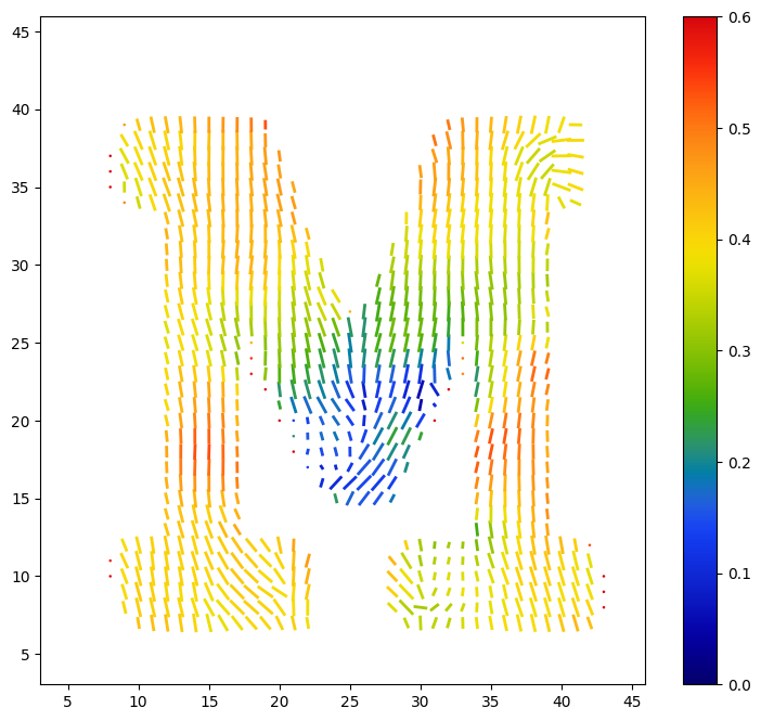
Based on these images, we will choose 0.4 and 1.0 as our cutoffs for the scale, and 0.2 and 1 as our cutoffs for the color. We check our reconstruction out using matplotlib.pyplot.quiver, which can also be a useful alternative to 3D rendering.

[18]:

scale_cutoff = (0.4, 1.0)
color_cutoff = (0.2, 1.)
test_scale = scale[5:45, 25, 5:45].clip(0, scale_cutoff[1])
test_scale[test_scale < scale_cutoff[0]] = np.nan
test_scale -= scale_cutoff[0]
test_scale /= (scale_cutoff[1] - scale_cutoff[0])
test_color = color[5:45, 25, 5:45].clip(*color_cutoff)
f, ax = plt.subplots(1, figsize=(9, 8))
x, y = np.meshgrid(np.arange(5, 45),
                   np.arange(5, 45),
                   indexing='ij')
test_orientation_x = orientation[5:45, 25, 5:45, 0] * test_scale
test_orientation_y = orientation[5:45, 25, 5:45, 2] * test_scale * np.sign(test_orientation_x)
test_orientation_x = abs(test_orientation_x)
q = ax.quiver(x, y, test_orientation_x, test_orientation_y,
              test_color, pivot='mid', angles='xy',
              headwidth=1, headlength=0, scale=30, width=0.005,
              cmap='cet_rainbow4', clim=color_cutoff)
plt.colorbar(q, ax=ax)
display(q)

<matplotlib.quiver.Quiver at 0x7f4f7ada3eb0>

../_images/tutorials_reconstruct_and_visualize_30_1.png

This concludes the tutorial.