Line segment integration

In this tutorial, you will learn how to change the integration paramters for the determination of the sphere-to-detector segment projection matrix, and see how modifying this property affects the segment-to-sphere mapping. At the end of the tutorial you will also see how this suppresses higher order terms when using the SphericalHarmonics basis set.

from mumott.methods.basis_sets import NearestNeighbor, GaussianKernels, SphericalHarmonics
from mumott.methods.utilities.grids_on_the_sphere import football
from mumott import ProbedCoordinates, SphericalHarmonicMapper
import numpy as np
from matplotlib import pyplot as plt
import colorcet

INFO:Setting the number of threads to 8. If your physical cores are fewer than this number, you may want to use numba.set_num_threads(n), and os.environ["OPENBLAS_NUM_THREADS"] = f"{n}" to set the number of threads to the number of physical cores n.
INFO:Setting numba log level to WARNING.

A key part of mumott is the mapping between detector segments and reciprocal space sphere. Typically, pixels along an arc on a detector are binned together to reduce data, which can be modelled by a line integral on the reciprocal space sphere. There are several ways to handle such line integrals. Either one can evaluate the integral using numerical quadrature until it converges (the default behaviour in mumott), or one can approximate the line integral by evaluating the central point of the line segment (the midpoint option in mumott). Both approaches can have advantages and disadvantages.

There are three quadrature rules that can be used in mumott:

• Simpson’s rule (simpson), the default, which interpolates order-2 polynomials and has a good tradeoff between complexity and accuracy. This is perhaps the most common numerical quadrature rule for accurate integrals.

• The Trapezoidal rule (trapezoid), which interpolates order-1 polynomials, and which can sometimes perform better than simpson.

• Romberg’s rule (romberg), which uses higher-order polynomials. It is a good all-around rule but more computationally intensive than simpson, and generally does not perform better.

Note: Generally, there is no reason to try one of the two other quadrature rules unless there are problems with attaining convergence using simpson.

SLERP

In SAXS, the line integrals lie on a great circle, and we can therefore use a SLERP to interpolate between endpoints, as well as to find midpoints. We will use this as a utility function in sketching out our line segment on the sphere, and to illustrate the effect we use a relatively large subtended angle, corresponding to binning a half-circle on the detector into approximately 3 segments.

vector = np.array([[0.5, 0, 0.25], [0.4, -0.18, -0.25]])
def slerp(t, vector):
    start = vector[0] / np.linalg.norm(vector[0])
    end = vector[-1] / np.linalg.norm(vector[-1])
    omega = np.arccos(np.sum(start * end))
    print(f'Subtended angle: {omega * 180 / np.pi} degrees')
    start = start.reshape(1, -1, 3)
    end = end.reshape(1, -1, 3)
    sin_omega = np.sin(omega)
    sin_tomega = np.sin(t * omega)
    sin_1mtomega = np.sin((1 - t) * omega)
    a = sin_1mtomega / sin_omega
    b = sin_tomega / sin_omega
    return a * start + b * end
vector_slerp = slerp(np.linspace(0, 1, 3).reshape(-1, 1), vector)
pc = ProbedCoordinates(vector=vector_slerp.reshape(1, 1, 3, 3))

Subtended angle: 60.84435669269466 degrees

segment_value = np.array([1.]).reshape(1, 1, 1, 1)

We want to evaluate the gradient contribution from this segment on a spherical grid, so we define a grid here.

n_points = 128
theta, phi = np.mgrid[0:np.pi+1e-6:np.pi/n_points, -np.pi/2:np.pi/2+1e-6:np.pi/n_points]
x, y, z = np.cos(phi) * np.sin(theta), np.sin(phi) * np.sin(theta), np.cos(theta)

Tip: If you do not know which basis set to use, then a reliable choice is GaussianKernels(grid_scale=number_of_segments // 2 + 1), and use the default quadrature rule, that is, ‘simpson’.

NearestNeighbor

The NearestNeighbor basis set bins the contribution from each point on the line segment into the closest point on a specified grid. It is probably the basis set where using the 'midpoint' rule makes the most sense, as it is difficult to get the line integral to converge. For this reason, the default tolerance of the line integral in NearestNeighbor is 1e-3 rather than the normal default of 1e-5.

bs = NearestNeighbor(football(), probed_coordinates=pc, integration_mode='midpoint')
grd = bs.gradient(segment_value)
directions = np.concatenate((x[..., None], y[..., None], z[..., None]), axis=-1).reshape(-1, 1, 1, 3)
amps_nn_midpoint = bs.get_amplitudes(grd, directions)

bs = NearestNeighbor(football(), probed_coordinates=pc, integration_maxiter=20)
grd = bs.gradient(segment_value)
directions = np.concatenate((x[..., None], y[..., None], z[..., None]), axis=-1).reshape(-1, 1, 1, 3)
amps_nn_simpson = bs.get_amplitudes(grd, directions)

GaussianKernels

Line integrals converge easily for GaussianKernels and perform well, and there is usually no particular reason to use 'midpoint' over a quadrature rule.

bs = GaussianKernels(grid_scale=5, probed_coordinates=pc, integration_mode='midpoint')
grd = bs.gradient(segment_value)
directions = np.concatenate((x[..., None], y[..., None], z[..., None]), axis=-1).reshape(-1, 1, 1, 3)
amps_gk_midpoint = bs.get_amplitudes(grd, ProbedCoordinates(directions))
norm_val = amps_gk_midpoint.max()
amps_gk_midpoint /= norm_val

bs = GaussianKernels(grid_scale=5, probed_coordinates=pc)
grd = bs.gradient(segment_value)
directions = np.concatenate((x[..., None], y[..., None], z[..., None]), axis=-1).reshape(-1, 1, 1, 3)
amps_gk_simpson = bs.get_amplitudes(grd, ProbedCoordinates(directions))
amps_gk_simpson /= norm_val

SphericalHarmonics

As with GaussianKernels, the line integrals easily converge for SphericalHarmonics, but will induce more anisotropy in ringing artefacts.

mapper = SphericalHarmonicMapper(ell_max=6, azimuthal_resolution=129 * 2, polar_resolution=129)
bs = SphericalHarmonics(ell_max=6, probed_coordinates=pc, integration_mode='midpoint')
grd = bs.gradient(segment_value)
amps_sh_midpoint = mapper.get_amplitudes(grd)[:, 65:-64]
norm_val = amps_sh_midpoint.max()
amps_sh_midpoint /= norm_val

bs = SphericalHarmonics(ell_max=6, probed_coordinates=pc)
grd = bs.gradient(segment_value)

amps_sh_simpson = mapper.get_amplitudes(grd)[:, 65:-64]
amps_sh_simpson /= norm_val

Evaluation

In order to plot the line, we define a SLERP, and then plot the sphere in a frontal view.

vector_slerp = slerp(np.linspace(0, 1, 10).reshape(-1, 1), vector)[0]

Subtended angle: 60.84435669269466 degrees

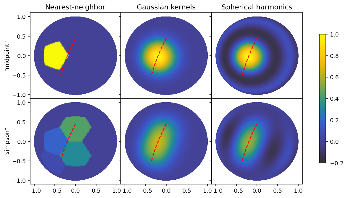
f, ax = plt.subplots(2, 3, figsize=(10.6, 5.4), dpi=140, sharex=True, sharey=True)
plt.subplots_adjust(wspace=0, hspace=0)
im = ax[0, 0].pcolormesh(y, z, amps_nn_midpoint.reshape((n_points + 1,) * 2), vmin=-0.2, vmax=1., shading='gouraud', cmap='cet_gouldian')
ax[1, 0].pcolormesh(y, z, amps_nn_simpson.reshape((n_points + 1,) * 2), vmin=-0.2, vmax=1., shading='gouraud', cmap='cet_gouldian')
ax[0, 1].pcolormesh(y, z, amps_gk_midpoint.reshape((n_points + 1,) * 2), vmin=-0.2, vmax=1., shading='gouraud', cmap='cet_gouldian')
ax[1, 1].pcolormesh(y, z, amps_gk_simpson.reshape((n_points + 1,) * 2), vmin=-0.2, vmax=1., shading='gouraud', cmap='cet_gouldian')
ax[0, 2].pcolormesh(mapper.unit_vectors[:, 65:-64, 1], mapper.unit_vectors[:, 65:-64, 2], amps_sh_midpoint.reshape((n_points + 1,) * 2), vmin=-0.2, vmax=1., shading='gouraud', cmap='cet_gouldian')
ax[1, 2].pcolormesh(mapper.unit_vectors[:, 65:-64, 1], mapper.unit_vectors[:, 65:-64, 2], amps_sh_simpson.reshape((n_points + 1,) * 2), vmin=-0.2, vmax=1., shading='gouraud', cmap='cet_gouldian')
for a in ax.ravel():
    a.set_xlim(-1.1, 1.1)
    a.set_ylim(-1.1, 1.1)
    a.plot(vector_slerp[:, 1], vector_slerp[:, 2], 'r--')
plt.colorbar(im, ax=ax, shrink=0.75)
ax[0, 0].set_title('Nearest-neighbor')
ax[0, 1].set_title('Gaussian kernels')
ax[0, 2].set_title('Spherical harmonics')
ax[0, 0].set_ylabel('"midpoint"')
ax[1, 0].set_ylabel('"simpson"')

Text(0, 0.5, '"simpson"')

Line segment length

This type of plot can also be useful when choosing a particular grid, resolution or ell_max, by plotting lines that subtend the same angle as the segments in your data with different parameters in your basis set. Broadly speaking, the midpoint rule is more useful when you have small segments relative to your basis set resolution, and the quadrature rules become more important as your basis set resolution grows larger. We can repeat this with a smaller line segment.

vector = np.array([[0.97, -0.10, 0.2],
                   [0.91, -0.3, -0.27]])
vector_slerp = slerp(np.linspace(0, 1, 3).reshape(-1, 1), vector)
pc = ProbedCoordinates(vector=vector_slerp.reshape(1, 1, 3, 3))

Subtended angle: 29.940725473859708 degrees

segment_value = np.array([1.]).reshape(1, 1, 1, 1)

n_points = 128
theta, phi = np.mgrid[0:np.pi+1e-6:np.pi/n_points, -np.pi/2:np.pi/2+1e-6:np.pi/n_points]
x, y, z = np.cos(phi) * np.sin(theta), np.sin(phi) * np.sin(theta), np.cos(theta)

We will now define the basis sets and compute amplitudes again.

bs = NearestNeighbor(football(), probed_coordinates=pc, integration_mode='midpoint')
grd = bs.gradient(segment_value)
directions = np.concatenate((x[..., None], y[..., None], z[..., None]), axis=-1).reshape(-1, 1, 1, 3)
amps_nn_midpoint = bs.get_amplitudes(grd, directions)

bs = NearestNeighbor(football(), probed_coordinates=pc, integration_maxiter=20)
grd = bs.gradient(segment_value)
directions = np.concatenate((x[..., None], y[..., None], z[..., None]), axis=-1).reshape(-1, 1, 1, 3)
amps_nn_simpson = bs.get_amplitudes(grd, directions)

bs = GaussianKernels(grid_scale=5, probed_coordinates=pc, integration_mode='midpoint')
grd = bs.gradient(segment_value)
directions = np.concatenate((x[..., None], y[..., None], z[..., None]), axis=-1).reshape(-1, 1, 1, 3)
amps_gk_midpoint = bs.get_amplitudes(grd, ProbedCoordinates(directions))
norm_val = amps_gk_midpoint.max()
amps_gk_midpoint /= norm_val

bs = GaussianKernels(grid_scale=5, probed_coordinates=pc)
grd = bs.gradient(segment_value)
directions = np.concatenate((x[..., None], y[..., None], z[..., None]), axis=-1).reshape(-1, 1, 1, 3)
amps_gk_simpson = bs.get_amplitudes(grd, ProbedCoordinates(directions))
amps_gk_simpson /= norm_val

mapper = SphericalHarmonicMapper(ell_max=6, azimuthal_resolution=129 * 2, polar_resolution=129)
bs = SphericalHarmonics(ell_max=6, probed_coordinates=pc, integration_mode='midpoint')
grd = bs.gradient(segment_value)
amps_sh_midpoint = mapper.get_amplitudes(grd)[:, 65:-64]
norm_val = amps_sh_midpoint.max()
amps_sh_midpoint /= norm_val

bs = SphericalHarmonics(ell_max=6, probed_coordinates=pc)
grd = bs.gradient(segment_value)

amps_sh_simpson = mapper.get_amplitudes(grd)[:, 65:-64]
amps_sh_simpson /= norm_val

vector_slerp = slerp(np.linspace(0, 1, 10).reshape(-1, 1), vector)[0]

Subtended angle: 29.940725473859708 degrees

f, ax = plt.subplots(2, 3, figsize=(10.6, 5.4), dpi=140, sharex=True, sharey=True)
plt.subplots_adjust(wspace=0, hspace=0)
im = ax[0, 0].pcolormesh(y, z, amps_nn_midpoint.reshape((n_points + 1,) * 2), vmin=-0.2, vmax=1., shading='gouraud', cmap='cet_gouldian')
ax[1, 0].pcolormesh(y, z, amps_nn_simpson.reshape((n_points + 1,) * 2), vmin=-0.2, vmax=1., shading='gouraud', cmap='cet_gouldian')
ax[0, 1].pcolormesh(y, z, amps_gk_midpoint.reshape((n_points + 1,) * 2), vmin=-0.2, vmax=1., shading='gouraud', cmap='cet_gouldian')
ax[1, 1].pcolormesh(y, z, amps_gk_simpson.reshape((n_points + 1,) * 2), vmin=-0.2, vmax=1., shading='gouraud', cmap='cet_gouldian')
ax[0, 2].pcolormesh(mapper.unit_vectors[:, 65:-64, 1], mapper.unit_vectors[:, 65:-64, 2], amps_sh_midpoint.reshape((n_points + 1,) * 2), vmin=-0.2, vmax=1., shading='gouraud', cmap='cet_gouldian')
ax[1, 2].pcolormesh(mapper.unit_vectors[:, 65:-64, 1], mapper.unit_vectors[:, 65:-64, 2], amps_sh_simpson.reshape((n_points + 1,) * 2), vmin=-0.2, vmax=1., shading='gouraud', cmap='cet_gouldian')
plt.colorbar(im, ax=ax, shrink=0.75)
for a in ax.ravel():
    a.set_xlim(-1.1, 1.1)
    a.set_ylim(-1.1, 1.1)
    a.plot(vector_slerp[:, 1], vector_slerp[:, 2], 'r--')
ax[0, 0].set_title('Nearest-neighbor')
ax[0, 1].set_title('Gaussian kernels')
ax[0, 2].set_title('Spherical harmonics')
ax[0, 0].set_ylabel('"midpoint"')
ax[1, 0].set_ylabel('"simpson"')

Text(0, 0.5, '"simpson"')

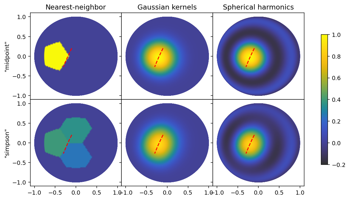
At this resolution, which is closer to a typical binning into 8 segments, the effect is far more subtle, and the choice only makes a big difference for the nearest-neighbor basis set, because the line segment happens to lie on an interface between three cells in the mesh.

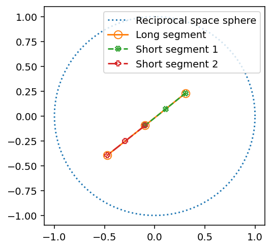
Weak additivity

One important distinction between the adaptive quadrature approaches, and the midpoint approximation, is that when doing quadrature, two adjacent line segments with equal values \(v_\text{half} + v_\text{half} = v_\text{sum}\) give the same gradient contribution as a single line segment with the value \(v_\text{sum}\). This is not true when using the midpoint approximation, and this weak additive property is useful to keep in mind even when deciding on how to reduce data.

vector = np.array([[0.6, 0.20, 0.15], [0.3, -0.18, -0.15]])
vector_1 = slerp(np.linspace(0, 1, 3).reshape(-1, 1), vector).reshape(1, 1, 3, 3)
vector_2 = slerp(np.array([0., 0.5, 1., 1., 1.5, 2.]).reshape(-1, 1) * 0.5, vector).reshape(1, 2, 3, 3)
vector_slerp = np.concatenate((vector_1, vector_2), axis=1)
pc = ProbedCoordinates(vector=vector_slerp.reshape(1, -1, 3, 3))

Subtended angle: 60.59015750182198 degrees
Subtended angle: 60.59015750182198 degrees

f, ax = plt.subplots(1, figsize=(4., 4.), dpi=140)
phi = np.linspace(0, np.pi * 2, 128)
x, y = np.cos(phi), np.sin(phi)
ax.plot(x, y, ':', label='Reciprocal space sphere')
ax.plot(vector_slerp[0, 0, :, 1], vector_slerp[0, 0, :, 2], 'o-', mfc='none', markersize=8, label='Long segment')
ax.plot(vector_slerp[0, 1, :, 1], vector_slerp[0, 1, :, 2], 'X--', mfc='none', markersize=5, label='Short segment 1')
ax.plot(vector_slerp[0, 2, :, 1], vector_slerp[0, 2, :, 2], 'P-.', mfc='none', markersize=5, label='Short segment 2')
ax.legend(loc='upper right')

<matplotlib.legend.Legend at 0x7f4567dbee90>

n_points = 128
theta, phi = np.mgrid[0:np.pi+1e-6:np.pi/n_points, -np.pi/2:np.pi/2+1e-6:np.pi/n_points]
x, y, z = np.cos(phi) * np.sin(theta), np.sin(phi) * np.sin(theta), np.cos(theta)

segment_value = np.array([1., 0., 0., 0., 0.5, 0.5]).reshape(2, 1, 1, 3)

We define basis sets again.

bs = GaussianKernels(grid_scale=8, probed_coordinates=pc, integration_mode='midpoint')
grd = bs.gradient(segment_value)
directions = np.concatenate((x[..., None], y[..., None], z[..., None]), axis=-1).reshape(-1, 1, 1, 3)
amps_gk_midpoint = bs.get_amplitudes(grd, ProbedCoordinates(directions))
norm_val = amps_gk_midpoint.max()

bs = GaussianKernels(grid_scale=8, probed_coordinates=pc)
grd = bs.gradient(segment_value)
directions = np.concatenate((x[..., None], y[..., None], z[..., None]), axis=-1).reshape(-1, 1, 1, 3)
amps_gk_simpson = bs.get_amplitudes(grd, ProbedCoordinates(directions))
norm_val = max(amps_gk_simpson.max(), norm_val)
amps_gk_midpoint /= norm_val
amps_gk_simpson /= norm_val

bs = NearestNeighbor(football(), probed_coordinates=pc, integration_mode='midpoint')
grd = bs.gradient(segment_value)
directions = np.concatenate((x[..., None], y[..., None], z[..., None]), axis=-1).reshape(-1, 1, 1, 3)
amps_nn_midpoint = bs.get_amplitudes(grd, directions)

bs = NearestNeighbor(football(), probed_coordinates=pc)
grd = bs.gradient(segment_value)
directions = np.concatenate((x[..., None], y[..., None], z[..., None]), axis=-1).reshape(-1, 1, 1, 3)
amps_nn_simpson = bs.get_amplitudes(grd, directions)

Here we also compute the spectral power of the spherical harmonic gradient, which will be useful in illustrating the higher-order attenuating effect of Simpson’s rule quadrature.

mapper = SphericalHarmonicMapper(ell_max=10, azimuthal_resolution=129 * 2, polar_resolution=129)
bs = SphericalHarmonics(ell_max=10, probed_coordinates=pc, integration_mode='midpoint')
grd = bs.gradient(segment_value)
amps_sh_midpoint_long = mapper.get_amplitudes(grd[0])[:, 65:-64]
norm_val_long = amps_sh_midpoint_long.max()
amps_sh_midpoint_short = mapper.get_amplitudes(grd[1])[:, 65:-64]
norm_val_short = amps_sh_midpoint_short.max()
spectrum_midpoint = bs.get_inner_product(grd, grd, resolve_spectrum=True)
bs = SphericalHarmonics(ell_max=10, probed_coordinates=pc)
grd = bs.gradient(segment_value)
spectrum_simpson = bs.get_inner_product(grd, grd, resolve_spectrum=True)

amps_sh_simpson_long = mapper.get_amplitudes(grd[0])[:, 65:-64]
norm_val_long_2 = amps_sh_simpson_long.max()
amps_sh_simpson_short = mapper.get_amplitudes(grd[1])[:, 65:-64]
norm_val_short_2 = amps_sh_simpson_short.max()
norm_val = np.max((norm_val_long, norm_val_short, norm_val_long_2, norm_val_short_2))
amps_sh_midpoint_long /= norm_val
amps_sh_midpoint_short /= norm_val
amps_sh_simpson_short /= norm_val
amps_sh_simpson_long /= norm_val

vector_slerp_long = slerp(np.linspace(0, 1, 10).reshape(-1, 1), vector).reshape(-1, 3)
vector_slerp_short_1 = slerp(np.linspace(0, 0.5, 3).reshape(-1, 1), vector).reshape(-1, 3)
vector_slerp_short_2 = slerp(np.linspace(0.5, 1, 3).reshape(-1, 1), vector).reshape(-1, 3)

Subtended angle: 60.59015750182198 degrees
Subtended angle: 60.59015750182198 degrees
Subtended angle: 60.59015750182198 degrees

f, ax = plt.subplots(4, 3, figsize=(10.6, 10.6), dpi=140, sharex=True, sharey=True)
plt.subplots_adjust(wspace=0, hspace=0)
im = ax[0, 0].pcolormesh(y, z, amps_nn_midpoint[0].reshape((n_points + 1,) * 2), vmin=-0.2, vmax=1., shading='gouraud', cmap='cet_gouldian')
ax[2, 0].pcolormesh(y, z, amps_nn_simpson[0].reshape((n_points + 1,) * 2), vmin=-0.2, vmax=1., shading='gouraud', cmap='cet_gouldian')
ax[0, 1].pcolormesh(y, z, amps_gk_midpoint[0].reshape((n_points + 1,) * 2), vmin=-0.2, vmax=1., shading='gouraud', cmap='cet_gouldian')
ax[2, 1].pcolormesh(y, z, amps_gk_simpson[0].reshape((n_points + 1,) * 2), vmin=-0.2, vmax=1., shading='gouraud', cmap='cet_gouldian')
ax[0, 2].pcolormesh(mapper.unit_vectors[:, 65:-64, 1], mapper.unit_vectors[:, 65:-64, 2], amps_sh_midpoint_long.reshape((n_points + 1,) * 2), vmin=-0.2, vmax=1., shading='gouraud', cmap='cet_gouldian')
ax[2, 2].pcolormesh(mapper.unit_vectors[:, 65:-64, 1], mapper.unit_vectors[:, 65:-64, 2], amps_sh_simpson_long.reshape((n_points + 1,) * 2), vmin=-0.2, vmax=1., shading='gouraud', cmap='cet_gouldian')

ax[1, 0].pcolormesh(y, z, amps_nn_midpoint[1].reshape((n_points + 1,) * 2), vmin=-0.2, vmax=1., shading='gouraud', cmap='cet_gouldian')
ax[3, 0].pcolormesh(y, z, amps_nn_simpson[1].reshape((n_points + 1,) * 2), vmin=-0.2, vmax=1., shading='gouraud', cmap='cet_gouldian')
ax[1, 1].pcolormesh(y, z, amps_gk_midpoint[1].reshape((n_points + 1,) * 2), vmin=-0.2, vmax=1., shading='gouraud', cmap='cet_gouldian')
ax[3, 1].pcolormesh(y, z, amps_gk_simpson[1].reshape((n_points + 1,) * 2), vmin=-0.2, vmax=1., shading='gouraud', cmap='cet_gouldian')
ax[1, 2].pcolormesh(mapper.unit_vectors[:, 65:-64, 1], mapper.unit_vectors[:, 65:-64, 2], amps_sh_midpoint_short.reshape((n_points + 1,) * 2), vmin=-0.2, vmax=1., shading='gouraud', cmap='cet_gouldian')
ax[3, 2].pcolormesh(mapper.unit_vectors[:, 65:-64, 1], mapper.unit_vectors[:, 65:-64, 2], amps_sh_simpson_short.reshape((n_points + 1,) * 2), vmin=-0.2, vmax=1., shading='gouraud', cmap='cet_gouldian')

plt.colorbar(im, ax=ax, shrink=0.75)
for i, a in enumerate(ax.ravel()):
    a.set_xlim(-1.1, 1.1)
    a.set_ylim(-1.1, 1.1)
    if i in (0, 1, 2, 6, 7, 8):
        a.plot(vector_slerp_long[:, 1], vector_slerp_long[:, 2], 'r--')
    else:
        a.plot(vector_slerp_short_1[:, 1], vector_slerp_short_1[:, 2], 'ko--')
        a.plot(vector_slerp_short_2[:, 1], vector_slerp_short_2[:, 2], 'm+--')
ax[0, 0].set_title('Nearest-neighbor')
ax[0, 1].set_title('Gaussian kernels')
ax[0, 2].set_title('Spherical harmonics')
ax[0, 0].set_ylabel('"midpoint", long')
ax[1, 0].set_ylabel('"midpoint", short')
ax[2, 0].set_ylabel('"simpson", long')
ax[3, 0].set_ylabel('"simpson", short')

Text(0, 0.5, '"simpson", short')

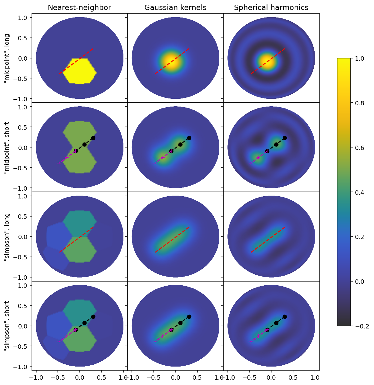
In all cases, the bottmo two rows are identical, since the two short segment values are equal in amplitude, and sum to the amplitude of the long segment. The shape of each gradient is similar to that of the second row (“midpoint”, short), but not identical, since the "midpoint" rule does not account for the extent of each shorter line, and because the resolution is relatively large compared to the segment length.

The top row, however, is completely different, since all the amplitude is binned into a single local impulse. This means that choosing a grid scale which is well adapted to the segment length is more crucial when using the "midpoint" rule. In addition, we can observer that the "midpoint" rule leads to a sparser matrix for the "NearestNeighbor" basis, which is in many cases desireable.

Finally we can observe that the "SphericalHarmonics" basis set has an attenuation in its ringing artefacts when the "midpoint". We can look at the spectral power function we computed earlier.

f, ax = plt.subplots(1, figsize=(2.8, 3.6), dpi=140)
ell = np.unique(bs.ell_indices)
ax.plot(ell, np.sqrt(spectrum_midpoint.squeeze()[0]), '^:', label='midpoint, long')
ax.plot(ell, np.sqrt(spectrum_midpoint.squeeze()[1]), 's-', label='midpoint, short')
ax.plot(ell, np.sqrt(spectrum_simpson.squeeze()[0]), 'o-.', label='simpson, long')
ax.plot(ell, np.sqrt(spectrum_simpson.squeeze()[1]), 'x--', label='simpson, short')
ax.set_ylim(0, 5)
ax.legend()
ax.set_xlabel(r'$\ell$')
ax.set_ylabel('Spectral amplitude')

Text(0, 0.5, 'Spectral amplitude')

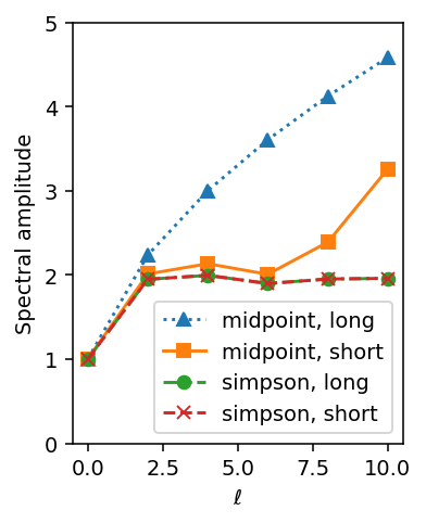
The difference between the midpoint rule and the integration rule for the shorter segments is smaller than that for the long case, but we see attenutation for \(\ell = 8\) and \(\ell = 10\) in particular; the effect is stronger at these higher frequencies because they exceed what we are normally able to resolve with this distance between probed points, and thus they undergo some attenuation when the integral is carried out. Therefore, when using the "midpoint" rule, it is a good idea to limit \(\ell_\text{max}\) or otherwise attenuate higher frequencies.