Zonal harmonics 2-step reconstruction workflow

This notebook shows how to use the Zonal Harmonics (ZH) reconstruction algorithm. The main difference between this algorithm and others implemented in mumott is that ZH assumes that the local scattering function in every pixel is axially symmetric around some axis parametrized by the polar coordinates, \(\theta_0\), \(\phi_0\). Each voxel can have a different axis of symmetry, and this axis is also found as a part of the optimization. The problem can be written as

\[c_{l0}, \theta_0, \phi_0 = \arg\min{\sum_{l,p,j,k}\Big|I - YPD(\theta_0, \phi_0)c_{l0}\Big|^2},\]

where \(I\) is the measured data, \(P\) is the usual projection matrix, \(Y\) are pre-computed sperical-harmonic functions, and \(D\) are Wigner’s D-matrices. Unlike other models used in mumott, this model is unavoidably non-convex since the forward model is non-linear in the two angle-parameters. Therefore, convergence to a global minimum cannot be guaranteed, and convergence to an appropriate solution will only occur if a good starting point for the angles is provided.

In this workflow we use a 2-step approach to the optimization, where first a different, convex, model is optimized. From this model, the symmetry-axis is calculated, and this axis is given as a starting point for a second optimization of the ZH model.

It is recommended to use GPU acceleration for this demonstration, as it is working with a high value of \(\ell_{\mathrm{max}}\) and therefore many spherical harmonics coefficients.

You first need to download the dataset from Zenodo, which can be accomplished on the command line as follows

wget https://zenodo.org/records/10408980/files/gamma_220.h5

The dataset comes from a tangled knot of hard-tempered steel wire using the austenite {220}-peak. The data consists of the integrated intensity of the full diffraciton peak in the radial direction and uses 48 azimuthal bins.

Imports

import matplotlib.pyplot as plt
import numpy as np
from mumott.data_handling import DataContainer
from mumott.methods.basis_sets import SphericalHarmonics
from mumott.methods.projectors import SAXSProjectorCUDA
from mumott.methods.residual_calculators import GradientResidualCalculator, ZHTTResidualCalculator
from mumott.optimization.loss_functions import SquaredLoss
from mumott.optimization.optimizers import LBFGS
from mumott.core.spherical_harmonic_mapper import SphericalHarmonicMapper
from mumott.methods.utilities.fiber_fit import find_approximate_symmetry_axis, degree_of_symmetry_map, symmetric_part_along_given_direction
from mumott.optimization.optimizers.zonal_harmonics_optimizer import ZHTTOptimizer

INFO:Setting the number of threads to 1. If your physical cores are fewer than this number, you may want to use numba.set_num_threads(n), and os.environ["OPENBLAS_NUM_THREADS"] = f"{n}" to set the number of threads to the number of physical cores n.
INFO:Setting numba log level to WARNING.

Initialize objects for first optimization

The workflow is compatible with any mumott reconstruction to generate the starting guess as long as it converges to a usable reconstruction from which the symmetry axis can be calculated.

This field defines a simple sperical-harmonics model without regularization and uses the LBFGS optimizer.

# Define a couple of parameters of the model.
ell_max_first_optimization = 10
maxiter_first_optimization = 10

data_container = DataContainer('gamma_220.h5', nonfinite_replacement_value = 0)

# The dataset contains a single bad frame liekly caused by a detector readout issue.
data_container.projections[166].data[46,58,:] = 0
data_container.projections[166].weights[46,58,:] = 0

basis_set = SphericalHarmonics(ell_max = ell_max_first_optimization)
projector = SAXSProjectorCUDA(data_container.geometry)
ResidualCalculator = GradientResidualCalculator(
                                data_container=data_container,
                                basis_set=basis_set,
                                projector=projector)
loss_function = SquaredLoss(ResidualCalculator, use_weights = True)
optimizer = LBFGS(loss_function, maxiter=maxiter_first_optimization)

INFO:Rotation matrices were loaded from the input file.

/das/home/carlse_m/mumott_dev_version/mumott/mumott/data_handling/data_container.py:227: DeprecationWarning: Entry name rotations is deprecated. Use inner_angle instead.
  _deprecated_key_warning('rotations')
/das/home/carlse_m/mumott_dev_version/mumott/mumott/data_handling/data_container.py:236: DeprecationWarning: Entry name tilts is deprecated. Use outer_angle instead.
  _deprecated_key_warning('tilts')
/das/home/carlse_m/mumott_dev_version/mumott/mumott/data_handling/data_container.py:268: DeprecationWarning: Entry name offset_j is deprecated. Use j_offset instead.
  _deprecated_key_warning('offset_j')
/das/home/carlse_m/mumott_dev_version/mumott/mumott/data_handling/data_container.py:278: DeprecationWarning: Entry name offset_k is deprecated. Use k_offset instead.
  _deprecated_key_warning('offset_k')

WARNING:The detector angles appear to cover a full circle. This is only expected for WAXS data.
INFO:Sample geometry loaded from file.
INFO:Detector geometry loaded from file.
INFO:Scattering angle loaded from data.

First optimization

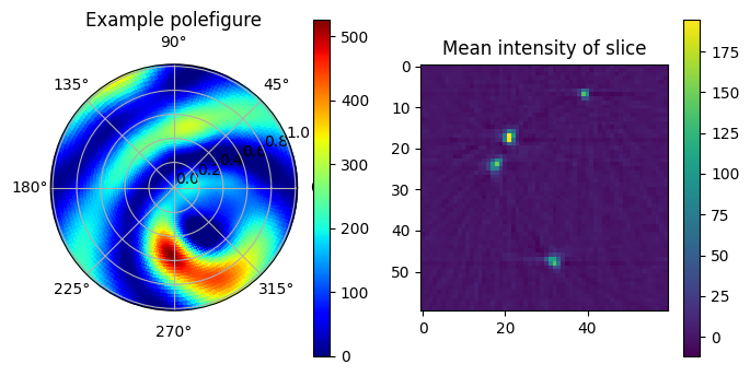
Here we perform the first-step optimization and plot an example slice and an example pole-figure from a single voxel and plot the results.

Note that we plot the scattering function in polar-coordinates in the stereoscopic projection, which is the convention in texture analysis. The central point of the figure is the \(z\)-axis and along the outer circle, \(\phi=0\) marks the \(x\)-axis and \(\phi=90^\circ\) marks the \(y\)-axis. Such a plot is commonly called a pole figure.

results = optimizer.optimize()
coefficients = basis_set.get_spherical_harmonic_coefficients(results['x'], ell_max=ell_max_first_optimization)

100%|███████████████████████████████████████████████████████████████████████████████████████████████████████████████████████████████████████████████████████████████████████████████████████████████████████████████████████████████████████████████████████████████████████████████████████| 10/10 [01:26<00:00,  8.68s/it]

# Choose a voxel that will be used in the plots of this notebook
example_index = (48, 25, 32)
pole_figure_resolution = 180

# Plot
mapper = SphericalHarmonicMapper(ell_max=ell_max_first_optimization,
                                 polar_resolution=pole_figure_resolution,
                                 azimuthal_resolution=pole_figure_resolution*2)
map = mapper.get_amplitudes(coefficients[(*example_index, slice(None))])

fig = plt.figure(figsize = (8,4))
ax = plt.subplot(1,2,1, polar=True)
img = ax.pcolormesh(mapper.phi[-1,:],
                    np.arctan(mapper.theta[:pole_figure_resolution//2, 0]/2),
                    map[:pole_figure_resolution//2],
                    edgecolors='face', cmap='jet')
plt.colorbar(img)
plt.title('Example polefigure')

plt.subplot(1,2,2)
plt.imshow(coefficients[:, 25, :, 0])
plt.colorbar()
plt.title('Mean intensity of slice')
plt.show()

Find approximate symmetry axis

The next step is to determine the symmetry axis from the first reconstruction. As can be seen in the previous plot, the pole figure contains two concentric rings, and the axis of symmetry is the center of these two rings.

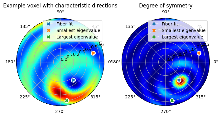
In general, to find the symmetry axis, we have two distinct approaches:

1. Calculate the eigenvectors from the 2nd order tensor component of the scattering function

2. Fit a rotationally symmetric function to the reconstructed function, and pick the axis with the best fit.

For systems with broad scattering features or a single direction with strong (or weak) scattering, it is recommmended to use the first approach. This is the case for samples such as bone, fiber-materials, and polycrystals with weak texture.

Since the eigenvector approach only uses the \(\ell = 2\) component, it does not perform well on systems where the high-\(\ell\) parts dominate, or where the \(\ell=2\) part vanishes. For such samples, the functions defined in mumott.methods.utilities.fiber_fit can be used instead.

To further emphasize the importance of the higher order components, the options filter='ramp' or filter='square' can be used. This can sometimes be helpful for noisy samples.

The best way to go about finding the axis is to inspect the plot below for a number of different representative voxels and see which of the two approaches and what parameters works best.

# Find symmetry axis by fitting (Icludes all ell)
fiberfit_gridsearch_resolution = 20  # Higher number means higher resolution
fit_zonal_harmonics, fit_theta, fit_phi \
    = find_approximate_symmetry_axis(coefficients, ell_max_first_optimization,
                                     fiberfit_gridsearch_resolution, filter = 'square')

# Find symmetry axis by tensor analysis (only ell = 2)
unrestricted_output = basis_set.get_output(coefficients)
main_eigenvector = unrestricted_output['spherical_functions']['eigenvectors'][..., 0]
tensor_theta = np.arccos(main_eigenvector[..., 2])
tensor_phi = np.arctan2(main_eigenvector[..., 1], main_eigenvector[..., 0])%(np.pi*2)

100%|███████████████████████████████████████████████████████████████████████████████████████████████████████████████████████████████████████████████████████████████████████████████████████████████████████████████████████████████████████████████████████████████████████████████████████| 10/10 [07:40<00:00, 46.00s/it]

############################### PLOT ######################
example_coeffs = coefficients[(*example_index, slice(None))]
mapper = SphericalHarmonicMapper(ell_max_first_optimization, pole_figure_resolution, pole_figure_resolution*2)
map = mapper.get_amplitudes(example_coeffs)
fiberfit_gridsearch_resolution_plot = 80  # Higher number means higher resolution

## SUBPLOT 1 ##
fig = plt.figure(figsize = (8,4))
ax = plt.subplot(1,2,1, polar=True)
plt.plot(fit_phi[example_index], np.arctan(fit_theta[example_index]/2),
         'wo', fillstyle = 'full', markersize = 10)
plt.plot(fit_phi[example_index], np.arctan(fit_theta[example_index]/2),
         'x', label = 'Fiber fit',markeredgewidth=3)
vector = unrestricted_output['spherical_functions']['eigenvectors'][(*example_index, slice(None), 0)]
vector = vector if vector[2] > 0 else -vector
theta = np.arccos(vector[2])
phi = np.arctan2(vector[1], vector[0])
plt.plot(phi, np.arctan(theta/2), 'wo', fillstyle = 'full', markersize = 10)
plt.plot(phi, np.arctan(theta/2), 'x', label = 'Smallest eigenvalue',markeredgewidth=3)
vector = unrestricted_output['spherical_functions']['eigenvectors'][(*example_index, slice(None), 2)]
vector = vector if vector[2] > 0 else -vector
theta = np.arccos(vector[2])
phi = np.arctan2(vector[1], vector[0])
plt.plot(phi, np.arctan(theta/2), 'wo', fillstyle = 'full', markersize = 10)
plt.plot(phi, np.arctan(theta/2), 'x', label = 'Largest eigenvalue',markeredgewidth=3)
plt.legend()
img = ax.pcolormesh(mapper.phi[-1,:],
                    np.arctan(mapper.theta[:pole_figure_resolution//2, 0]/2),
                    map[:pole_figure_resolution//2], edgecolors='face', cmap='jet')
plt.title('Example voxel with characteristic directions')

## SUBPLOT 2 ##
ax = plt.subplot(1,2,2, polar=True)
plt.plot(fit_phi[example_index], np.arctan(fit_theta[example_index]/2), 'wo', fillstyle = 'full', markersize = 10)
plt.plot(fit_phi[example_index], np.arctan(fit_theta[example_index]/2), 'x', label = 'Fiber fit',markeredgewidth=3)
vector = unrestricted_output['spherical_functions']['eigenvectors'][(*example_index, slice(None), 0)]
vector = vector if vector[2] > 0 else -vector
theta = np.arccos(vector[2])
phi = np.arctan2(vector[1], vector[0])
plt.plot(phi, np.arctan(theta/2), 'wo', fillstyle = 'full', markersize = 10)
plt.plot(phi, np.arctan(theta/2), 'x', label = 'Smallest eigenvalue',markeredgewidth=3)
vector = unrestricted_output['spherical_functions']['eigenvectors'][(*example_index, slice(None), 2)]
vector = vector if vector[2] > 0 else -vector
theta = np.arccos(vector[2])
phi = np.arctan2(vector[1], vector[0])
plt.plot(phi, np.arctan(theta/2), 'wo', fillstyle = 'full', markersize = 10)
plt.plot(phi, np.arctan(theta/2), 'x', label = 'Largest eigenvalue',markeredgewidth=3)
plt.legend()
map, map_theta, map_phi = degree_of_symmetry_map(example_coeffs, ell_max_first_optimization,
                                                 fiberfit_gridsearch_resolution_plot, filter = 'square')
img = ax.pcolormesh(map_phi[:fiberfit_gridsearch_resolution_plot//2],
                    np.arctan(map_theta[:fiberfit_gridsearch_resolution_plot//2]/2),
                    map[:fiberfit_gridsearch_resolution_plot//2], edgecolors='face', cmap='jet')
plt.title('Degree of symmetry')
plt.show()

Choose a direction and calculate the best-fit symmetric coefficients

After inspecting the previous figure, we see that the Fiber fit calculation finds the symmetry axis while the eigenvectors instead find the middle of the strongest diffraction feature, and a direction orthogonal to this.

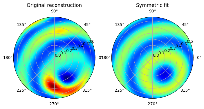
In the next code block we therefore choose to proceed with the fitted angles, and to calculate the best-fit zonal coefficients along this direction which we will use as the initial condition for the second optimization.

We also need to choose the \(\ell_{\mathrm{max}}\) parameter for the ZH model, which determines the angular resolution of the reconstruction. One should not choose a \(\ell_{\mathrm{max}}\) larger than half the number of azimuthal bins in the data set, and one also has to be aware that choosing a large value will use a lot of memory on the computer and slow down the calculation.

# Here you need to choose which directions to use
init_theta, init_phi = fit_theta, fit_phi
#init_theta, init_phi = tensor_theta, tensor_phi

# Calculate the zonal harmonics along chosen directions
ell_max_second_optimization = 20
padded_coefficients = basis_set.get_spherical_harmonic_coefficients(results['x'], ell_max=ell_max_second_optimization)
zonal_coefficients = symmetric_part_along_given_direction(padded_coefficients, init_theta, init_phi,
                                                          ell_max=ell_max_second_optimization)

#################################### PLOT ##################################
basis_set = SphericalHarmonics(ell_max = ell_max_second_optimization)
zzh_forward_model = ZHTTResidualCalculator(data_container=data_container,
                                           basis_set=basis_set,
                                           projector=projector)

zzh_forward_model.coefficients = np.concatenate((zonal_coefficients,
                                                 init_theta[..., np.newaxis],
                                                 init_phi[..., np.newaxis]), axis = -1)
sym_function_full_coeffs = zzh_forward_model.rotated_coefficients
mapper = SphericalHarmonicMapper(ell_max_second_optimization, pole_figure_resolution, pole_figure_resolution*2)
map = mapper.get_amplitudes(padded_coefficients[(*example_index, slice(None))])
sym_map = mapper.get_amplitudes(sym_function_full_coeffs[(*example_index, slice(None))])

fig = plt.figure(figsize=(8,4))
ax = plt.subplot(1,2,1, polar=True)
img = ax.pcolormesh(mapper.phi[-1,:],
                    np.arctan(mapper.theta[:pole_figure_resolution//2, 0]/2),
                    map[:pole_figure_resolution//2],
                    edgecolors='face', cmap='jet',vmin=np.min(map), vmax=np.max(map))
ax.set_title('Original reconstruction')
ax = plt.subplot(1,2,2, polar=True)
img = ax.pcolormesh(mapper.phi[-1,:],
                    np.arctan(mapper.theta[:pole_figure_resolution//2, 0]/2),
                    sym_map[:pole_figure_resolution//2],
                    edgecolors='face', cmap='jet',vmin=np.min(map), vmax=np.max(map))
ax.set_title('Symmetric fit')
plt.show()

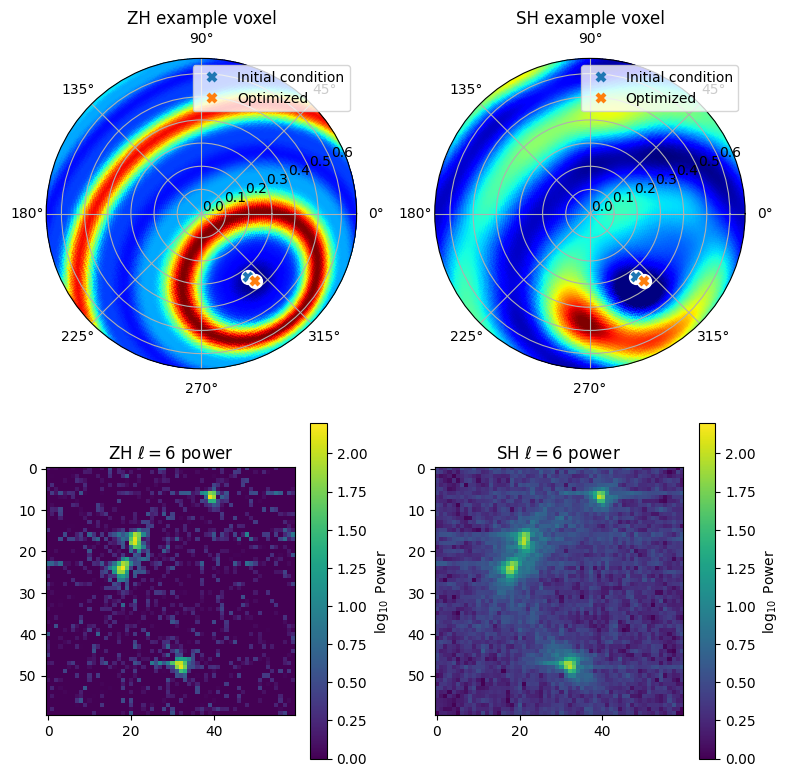
Fit the symmetric model

Now all the setup is done and we are ready to do the optimization of the ZH model.

The optimizer currently implemented is a simple gradient-descent algorithms with a heuristic rule determining the step size for the angle degrees of freedom. It has relatively slow convergence for the angles, so use a large number of iterations to be safe.

# Set parameters for the ZH model and optimization
maxiter_second_optimization = 30

start_paramters = np.ascontiguousarray(np.concatenate((zonal_coefficients, init_theta[..., np.newaxis], init_phi[..., np.newaxis]), axis = -1)).astype(projector.dtype)
basis_set = SphericalHarmonics(ell_max = ell_max_second_optimization)
zzh_forward_model = ZHTTResidualCalculator(data_container=data_container,
                                           basis_set=basis_set,
                                           projector=projector)
loss_function = SquaredLoss(zzh_forward_model, use_weights = True)
optimizer = ZHTTOptimizer(loss_function, start_paramters, maxiter=maxiter_second_optimization)
result = optimizer.optimize()

INFO:Since the step size has not been specified the largest safe step size will beestimated. This calculation is approximate and does not take into accountregularization. There is therefore no guarantee of convergence.

Loss = 1.49E+11: 100%|██████████████████████████████████████████████████████████████████████████████████████████████████████████████████████████████████████████████████████████████████████████████████████████████████████████████████████████████████████████████████████████████████████| 30/30 [13:51<00:00, 27.72s/it]

##################### PLOT #################################
zzh_forward_model.coefficients = result['x']
example_coeffs = zzh_forward_model.rotated_coefficients[(*example_index, slice(None))]
theta_zh = zzh_forward_model._theta[example_index]
phi_zh = zzh_forward_model._phi[example_index]
mapper = SphericalHarmonicMapper(ell_max_second_optimization, pole_figure_resolution, pole_figure_resolution*2)
sym_map = mapper.get_amplitudes(example_coeffs)

### Plot pole figures ###
fig = plt.figure(figsize = (8,8))
ax = plt.subplot(2,2,1, polar=True)
plt.plot(init_phi[example_index], np.arctan(init_theta[example_index]/2), 'wo',
         fillstyle = 'full', markersize = 10)
plt.plot(init_phi[example_index], np.arctan(init_theta[example_index]/2), 'x',
         label = 'Initial condition',markeredgewidth=3)
plt.plot(phi_zh, np.arctan(theta_zh/2), 'wo', fillstyle = 'full', markersize = 10)
plt.plot(phi_zh, np.arctan(theta_zh/2), 'x', label = 'Optimized',markeredgewidth=3)
plt.legend()
img = ax.pcolormesh(mapper.phi[-1,:],
                    np.arctan(mapper.theta[:pole_figure_resolution//2, 0]/2),
                    sym_map[:pole_figure_resolution//2],
                    edgecolors='face', cmap='jet',vmin=np.min(sym_map), vmax=np.max(sym_map))
plt.title('ZH example voxel')
ax = plt.subplot(2,2,2, polar=True)
plt.plot(init_phi[example_index], np.arctan(init_theta[example_index]/2), 'wo',
         fillstyle = 'full', markersize = 10)
plt.plot(init_phi[example_index], np.arctan(init_theta[example_index]/2), 'x',
         label = 'Initial condition',markeredgewidth=3)
plt.plot(phi_zh, np.arctan(theta_zh/2), 'wo', fillstyle = 'full', markersize = 10)
plt.plot(phi_zh, np.arctan(theta_zh/2), 'x', label = 'Optimized',markeredgewidth=3)
plt.legend()
img = ax.pcolormesh(mapper.phi[-1,:],
                    np.arctan(mapper.theta[:pole_figure_resolution//2, 0]/2),
                    map[:pole_figure_resolution//2],
                    edgecolors='face', cmap='jet',vmin=np.min(sym_map), vmax=np.max(sym_map))
plt.title('SH example voxel')

### PLot slices ###
plt.subplot(2,2,3)
plt.imshow(np.abs(zzh_forward_model.coefficients[:,25,:, 3]))
plt.colorbar()
plt.title(r'ZH $\ell=6$ power')
plt.subplot(2,2,4)
plt.imshow(np.linalg.norm(coefficients[:,25,:, 15:28], axis = -1))
plt.colorbar()
plt.title(r'SH $\ell=6$ power')
plt.tight_layout()
plt.show()

Generate output

The results can be obtained in the form of an output dictionary in the usual way by the get_output() method of the basis_set, except the method residual_calculator.rotated_coefficients has to be called to generate coefficients in the correct format.

Furthermore, the symmetry axis is not known by the basis_set, so this has to be added to the output dictionary manually.

The zzh_forward_model.coefficients property is used here, because behind the scenes, it casts all the angles to lie in the first symmetric zone \(\theta\in [0, \pi/2]\) and \(\phi\in [0, 2\pi [\). The angles could have drifted out of this region during the optimization and ended up in a symmetry equivalent point.

zzh_forward_model.coefficients = result['x']
symmetric_solution_full_basis = zzh_forward_model.rotated_coefficients
nicer_parameters = zzh_forward_model.coefficients

output = basis_set.get_output(coefficients = zzh_forward_model.rotated_coefficients)
output['theta'] = nicer_parameters[..., -2]
output['phi'] = nicer_parameters[..., -1]
output['zonal_coefficients'] = nicer_parameters[..., :-2]
output['main_direction'] = zzh_forward_model.directions