Asynchronous reconstruction
This tutorial demonstrates the pipelines for spherical integral geometric tensor tomography (SIRT) and the modular iterative tomographic reconstruction algorithm (MITRA), and how they can be used to get started with a reconstruction quickly.
The dataset of trabecular bone used in this tutorial is available via Zenodo, and can be downloaded either via a browser or the command line using, e.g., wget or curl,
wget https://zenodo.org/records/10074598/files/trabecular_bone_9.h5
[1]:
import warnings
from mumott.data_handling import DataContainer
from mumott.methods.basis_sets import GaussianKernels
from mumott.pipelines.async_pipelines import run_motr, run_tensor_sirt, run_radtt
import matplotlib.pyplot as plt
import colorcet
import logging
import numpy as np
data_container = DataContainer('trabecular_bone_9.h5')
INFO:Setting the number of threads to 4. If your physical cores are fewer than this number, you may want to use numba.set_num_threads(n), and os.environ["OPENBLAS_NUM_THREADS"] = f"{n}" to set the number of threads to the number of physical cores n.
INFO:Setting numba log level to WARNING.
INFO:Inner axis found in dataset base directory. This will override the default.
INFO:Outer axis found in dataset base directory. This will override the default.
INFO:Rotation matrices were loaded from the input file.
INFO:Sample geometry loaded from file.
INFO:Detector geometry loaded from file.
Asynchronous Tensor SIRT
The Tensor SIRT asynchronous pipeline is similar to the synchronous pipeline MITRA. It computes a preconditioner and weight set based on the basis set and projection geometry. However, it does not used momentum acceleration for convergence, and does not use any regularization - the only hyperparameter for the optimization is the number of iterations.
This is a good use-case for asynchronous reconstruction, since the algorithm is very simple, and benefits from the large speedup.
[2]:
%%time
results = run_tensor_sirt(data_container,
                          maxiter=50,
                          update_frequency=25)
reconstruction = results['reconstruction']
basis_set = results['basis_set']
output = basis_set.get_output(reconstruction)
100%|██████████| 50/50 [00:16<00:00,  3.09it/s]
CPU times: user 24.4 s, sys: 861 ms, total: 25.3 s
Wall time: 26.4 s
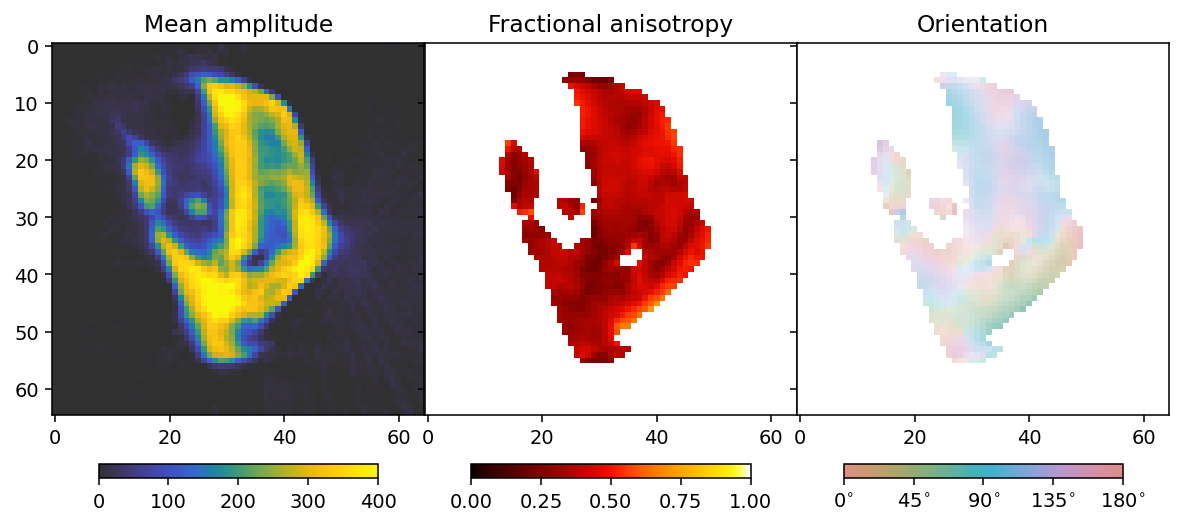
To analyze the results we here define a convenience function that allows us to extract mean, fractional anisotropy, and orientation data in a 2D slice from the reconstruction.
The function defined here uses output.eigenvector_1 which corresponds to the direction with lowest scattering, For equatorial ring type scattering output.eigenvector_1 is apropriate. For polar cap type scattering, output.eigenvector_3.
[3]:
plotted_slice_index = 28
mask_threshold = 100

def get_2d_images(output):

    mean = output.mean_intensity[plotted_slice_index]
    mask = mean > mask_threshold

    fractional_anisotropy = output.fractional_anisotropy[plotted_slice_index]
    fractional_anisotropy[~mask] = 1

    main_eigenvector = output.eigenvector_1[plotted_slice_index]
    orientation = np.arctan2(-main_eigenvector[..., 1],
                             main_eigenvector[..., 2])
    orientation[orientation < 0] += np.pi
    orientation[orientation > np.pi] -= np.pi
    orientation *= 180 / np.pi

    alpha = np.clip(output.fractional_anisotropy[plotted_slice_index], 0, 1)
    alpha[~mask] = 0

    return mean, fractional_anisotropy, orientation, alpha
[4]:
mean, fractional_anisotropy, orientation, alpha = get_2d_images(output)
Next we plot the results.
[5]:
colorbar_kwargs = dict(orientation='horizontal', shrink=0.75, pad=0.1)
mean_kwargs = dict(vmin=0, vmax=400, cmap='cet_gouldian')
fractional_anisotropy_kwargs = dict(vmin=0, vmax=1.0, cmap='cet_fire')
orientation_kwargs = dict(vmin=0, vmax=180, cmap='cet_CET_C10')

def config_cbar(cbar):
    cbar.set_ticks([i for i in np.linspace(0, 180, 5)])
    cbar.set_ticklabels([r'$' + f'{int(v):d}' + r'^{\circ}$' for v in bar.get_ticks()])
[6]:
fig, ax = plt.subplots(1, 3, figsize=(10.3, 4.6), dpi=140, sharey=True)


im0 = ax[0].imshow(mean, **mean_kwargs);
im1 = ax[1].imshow(fractional_anisotropy, **fractional_anisotropy_kwargs);
im2 = ax[2].imshow(orientation, alpha=alpha, **orientation_kwargs);

ax[0].set_title('Mean amplitude')
ax[1].set_title('Fractional anisotropy')
ax[2].set_title('Orientation')

plt.subplots_adjust(wspace=0)

plt.colorbar(im0, ax=ax[0], **colorbar_kwargs)
plt.colorbar(im1, ax=ax[1], **colorbar_kwargs)
bar = plt.colorbar(im2, ax=ax[2], **colorbar_kwargs)
config_cbar(bar)
MOTR - Momentum-accelerated Total variation Reconstruction
MOTR is similar to MITRA with the TV and Huber Norm regularizers used. However, the asynchronus TV and L1 regularizers are simpler - they do not have a delta term for small terms, and may therefore require more careful adjustment of the step size if a particular degree of convergence is to be obtained, especialy if the regularization weights are large. Generally, however, they can be used in much the same way.
[7]:
%%time
beta_values = np.geomspace(0.5, 5, 3)
result = []
values = []
for beta in beta_values:
    result.append(run_motr(data_container,
                           maxiter=30,
                           l1_weight=0.,
                           tv_weight=beta,
                           update_frequency=15))
    values.append(beta)
Loss: 1.88e+10 Res.norm: 1.84e+10 L1 norm: 6.74e+08 TV norm: 7.16e+08: 100%|██████████| 30/30 [00:12<00:00,  2.46it/s]
Loss: 2.31e+10 Res.norm: 2.22e+10 L1 norm: 5.99e+08 TV norm: 6.05e+08: 100%|██████████| 30/30 [00:12<00:00,  2.46it/s]
Loss: 3.73e+10 Res.norm: 3.32e+10 L1 norm: 6.41e+08 TV norm: 8.34e+08: 100%|██████████| 30/30 [00:12<00:00,  2.45it/s]
CPU times: user 44.8 s, sys: 2.37 s, total: 47.2 s
Wall time: 45.7 s
[8]:
reconstructions = [r['reconstruction'] for r in result]
outputs = [r['basis_set'].get_output(r['reconstruction']) for r in result]
/das/home/carlse_m/p20850/envs/mumott_latest/lib/python3.11/site-packages/mumott/methods/basis_sets/gaussian_kernels.py:490: RuntimeWarning: invalid value encountered in divide
  fractional_anisotropy = fractional_anisotropy / np.sqrt(2*np.sum(eigenvalues**2, axis=-1))
[9]:
colorbar_kwargs = dict(orientation='horizontal', shrink=0.75, pad=0.033)
fig, axes = plt.subplots(3, 3, figsize=(9.4, 11.6), dpi=140, sharey=True, sharex=True)
for i in range(3):
    ax = axes[i]
    mean, fractional_anisotropy, orientation, alpha = get_2d_images(outputs[i])
    plt.subplots_adjust(wspace=0, hspace=0)
    im0 = ax[0].imshow(mean, **mean_kwargs);
    im1 = ax[1].imshow(fractional_anisotropy, **fractional_anisotropy_kwargs);
    im2 = ax[2].imshow(orientation, alpha=alpha, **orientation_kwargs);
    if i == 0:
        ax[0].set_title('Mean amplitude')
        ax[1].set_title('Fractional anisotropy')
        ax[2].set_title('Orientation')
    ax[0].set_ylabel(r'$\beta = ' + f'{beta_values[i]:.2f}' + r'$')
    if i == 2:
        plt.colorbar(im0, ax=axes[:, 0], **colorbar_kwargs);
        plt.colorbar(im1, ax=axes[:, 1], **colorbar_kwargs);
        bar = plt.colorbar(im2, ax=axes[:, 2], **colorbar_kwargs);
        config_cbar(bar)
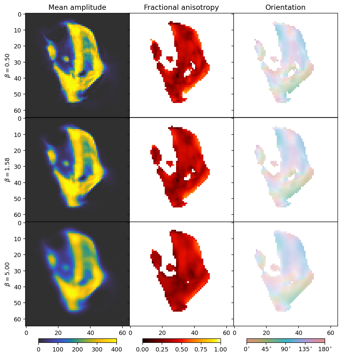
As before with increasing beta, the reconstructions become blurrier. The comparison suggests that a suitable choice for beta should be between the first and second row.
Next we scan different values for alpha (L1) with beta=1 (total variation).
[10]:
%%time
alpha_values = np.geomspace(1, 40, 3)
result = []
values = []
for alpha in alpha_values:
    result.append(run_motr(data_container,
                           maxiter=30,
                           l1_weight=alpha,
                           tv_weight=1.,
                           update_frequency=15))
    values.append(alpha)
Loss: 2.41e+10 Res.norm: 2.31e+10 L1 norm: 4.35e+08 TV norm: 5.86e+08: 100%|██████████| 30/30 [00:12<00:00,  2.45it/s]
Loss: 3.42e+10 Res.norm: 3.07e+10 L1 norm: 4.36e+08 TV norm: 7.08e+08: 100%|██████████| 30/30 [00:12<00:00,  2.46it/s]
Loss: 6.25e+11 Res.norm: 5.81e+11 L1 norm: 1.06e+09 TV norm: 1.98e+09: 100%|██████████| 30/30 [00:12<00:00,  2.46it/s]
CPU times: user 44.9 s, sys: 2.09 s, total: 47 s
Wall time: 45.4 s
[11]:
reconstructions = [r['reconstruction'] for r in result]
outputs = [r['basis_set'].get_output(r['reconstruction']) for r in result]
/das/home/carlse_m/p20850/envs/mumott_latest/lib/python3.11/site-packages/mumott/methods/basis_sets/gaussian_kernels.py:490: RuntimeWarning: invalid value encountered in divide
  fractional_anisotropy = fractional_anisotropy / np.sqrt(2*np.sum(eigenvalues**2, axis=-1))
[12]:
fig, axes = plt.subplots(3, 3, figsize=(9.4, 11.6), dpi=140, sharey=True, sharex=True)
for i in range(3):
    ax = axes[i]
    mean, fractional_anisotropy, orientation, alpha = get_2d_images(outputs[i])
    plt.subplots_adjust(wspace=0, hspace=0)
    im0 = ax[0].imshow(mean, **mean_kwargs);
    im1 = ax[1].imshow(fractional_anisotropy, **fractional_anisotropy_kwargs);
    im2 = ax[2].imshow(orientation, alpha=alpha, **orientation_kwargs);
    if i == 0:
        ax[0].set_title('Mean amplitude')
        ax[1].set_title('Fractional anisotropy')
        ax[2].set_title('Orientation')
    ax[0].set_ylabel(r'$\alpha = ' + f'{alpha_values[i]:.2f}' + r'$')
    if i == 2:
        plt.colorbar(im0, ax=axes[:, 0],  **colorbar_kwargs);
        plt.colorbar(im1, ax=axes[:, 1],  **colorbar_kwargs);
        bar = plt.colorbar(im2, ax=axes[:, 2],  **colorbar_kwargs);
        config_cbar(bar)
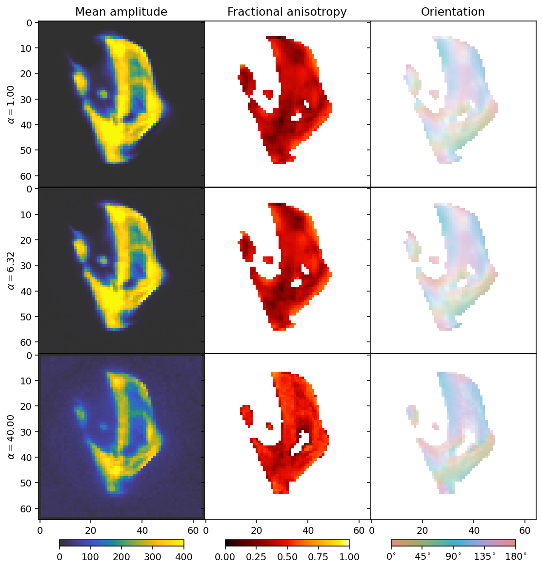
We can now see the effect of the \(L_1\) regularizer. It has a broad dampening effect that first only acts on the background, but eventually becomes strong enough to dampen the entire reconstruction.
The comparison suggests a value for alpha somewhere around 6 (middle row), showing that the result is quite similar as for the synchronous Huber Norm. We see a slightly different behaviour for the background as by default, run_motr is thresholded so that coefficients cannot have values smaller than zero. We might therefore want to pick the regularization weight that has just the right size to zero out the background, being neither too large nor too small.
RADTT - Huber-TV reconstruction
One of the advantages of asynchronous reconstruction is that we can use a far greater number of iterations, due to the speedup. This allows us to use algorithms that take longer to converge or requires more hyperparameters to be figured out. For example, an optimization that uses the Huber norm can be a very robust way to reconstruct a data set with outliers, but the optimal step size is difficult to figure out. We will add some random, high-intensity artefacts to the data to illustrate the advantages of robust optimization.
[13]:
data_container = DataContainer('trabecular_bone_9.h5')
seed = 123456
rng = np.random.default_rng(seed)
for p in data_container.projections:
    inds_1, inds_2, inds_3 = np.unravel_index(rng.choice(p.data.size, 5000, replace=False), p.data.shape)
    for (i, j, k) in zip(inds_1, inds_2, inds_3):
        p.data[i, j, k] += rng.laplace(1e4, 0.5e4)
    inds_1, inds_2, inds_3 = np.unravel_index(rng.choice(p.data.size, 50, replace=False), p.data.shape)
    for (i, j, k) in zip(inds_1, inds_2, inds_3):
        p.data[i, j, k] += rng.laplace(1e5, 0.2e5)
INFO:Inner axis found in dataset base directory. This will override the default.
INFO:Outer axis found in dataset base directory. This will override the default.
INFO:Rotation matrices were loaded from the input file.
INFO:Sample geometry loaded from file.
INFO:Detector geometry loaded from file.
We will see the influence of the noise by doing a tensor SIRT reconstruction.
[14]:
results = run_tensor_sirt(data_container,
                          maxiter=50,
                          update_frequency=25)
reconstruction = results['reconstruction']
basis_set = results['basis_set']
output = basis_set.get_output(reconstruction)
100%|██████████| 50/50 [00:16<00:00, 3.09it/s]
[15]:
mean, fractional_anisotropy, orientation, alpha = get_2d_images(output)
fig, ax = plt.subplots(1, 3, figsize=(10.3, 4.6), dpi=140, sharey=True)

im0 = ax[0].imshow(mean, **mean_kwargs);
im1 = ax[1].imshow(fractional_anisotropy, **fractional_anisotropy_kwargs);
im2 = ax[2].imshow(orientation, alpha=alpha, **orientation_kwargs);

ax[0].set_title('Mean amplitude')
ax[1].set_title('Fractional anisotropy')
ax[2].set_title('Orientation')

plt.subplots_adjust(wspace=0)

plt.colorbar(im0, ax=ax[0], **colorbar_kwargs)
plt.colorbar(im1, ax=ax[1], **colorbar_kwargs)
bar = plt.colorbar(im2, ax=ax[2], **colorbar_kwargs)
config_cbar(bar)
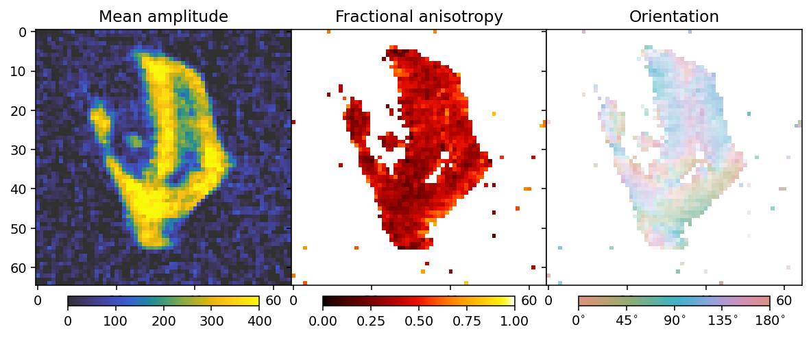
This does not look very good compared to the appearance of the data without the noise at the beginning of this tutorial notebook, but we will see that RADTT can still perform well.
To use the robust reconstruction pipeline, we need to first figure out a step size. We will use some descriptive statistics of the data to inform our guess.
[16]:
percentiles = np.linspace(0, 99.9, 1000)
values = np.percentile(data_container.data, percentiles)
f, ax = plt.subplots(1, 1, figsize=(4, 3), dpi=140)
ax.semilogy(percentiles, values)
ax.set_ylabel('Data')
ax.set_xlabel('Percentile')
[16]:
Text(0.5, 0, 'Percentile')
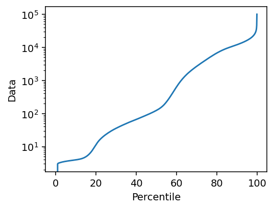
We know that the data contains both background (below 20th percentile) and a PMMA substrate (below 60th percentile), as well as directions which do not scatter very much, and these are not very relevant to the step size. Thus we choose a value close to the upper end of the distribution, at the 80th percentile. We then try a range of step sizes.
[17]:
%%time
reference_value = np.percentile(data_container.data, 80)
step_sizes = np.geomspace(1e-3, 1, 5)
results = []
for s in step_sizes:
    results.append(run_radtt(data_container,
                             step_size=s * reference_value,
                             delta=0.,
                             tv_weight=0.,
                             maxiter=50,
                             update_frequency=10))
Loss: 5.06e+12 Res.norm: 5.06e+12 TV norm: 5.53e+07: 100%|██████████| 50/50 [00:21<00:00,  2.35it/s]
Loss: 4.16e+12 Res.norm: 4.16e+12 TV norm: 1.83e+08: 100%|██████████| 50/50 [00:21<00:00,  2.35it/s]
Loss: 3.66e+12 Res.norm: 3.66e+12 TV norm: 4.34e+08: 100%|██████████| 50/50 [00:20<00:00,  2.38it/s]
Loss: 3.62e+12 Res.norm: 3.62e+12 TV norm: 7.10e+08: 100%|██████████| 50/50 [00:20<00:00,  2.40it/s]
Loss: 3.68e+12 Res.norm: 3.68e+12 TV norm: 1.02e+09: 100%|██████████| 50/50 [00:20<00:00,  2.42it/s]
CPU times: user 1min 56s, sys: 5.69 s, total: 2min 1s
Wall time: 1min 59s
[18]:
reconstructions = [r['reconstruction'] for r in results]
outputs = [r['basis_set'].get_output(r['reconstruction']) for r in results]
loss = [r['loss_curve'][-1][1] for r in results]
/das/home/carlse_m/p20850/envs/mumott_latest/lib/python3.11/site-packages/mumott/methods/basis_sets/gaussian_kernels.py:490: RuntimeWarning: invalid value encountered in divide
  fractional_anisotropy = fractional_anisotropy / np.sqrt(2*np.sum(eigenvalues**2, axis=-1))
[19]:
fig, axes = plt.subplots(5, 3, figsize=(9.4, 15.6), dpi=140, sharey=True, sharex=True)
for i in range(5):
    ax = axes[i]
    mean, fractional_anisotropy, orientation, alpha = get_2d_images(outputs[i])
    plt.subplots_adjust(wspace=0, hspace=0)
    im0 = ax[0].imshow(mean, **mean_kwargs);
    im1 = ax[1].imshow(fractional_anisotropy, **fractional_anisotropy_kwargs);
    im2 = ax[2].imshow(orientation, alpha=alpha, **orientation_kwargs);
    if i == 0:
        ax[0].set_title('Mean amplitude')
        ax[1].set_title('Fractional anisotropy')
        ax[2].set_title('Orientation')
    ax[0].set_ylabel(r'$stepsize = ' + f'{step_sizes[i]:.2f}' + r'$')
    if i == 4:
        plt.colorbar(im0, ax=axes[:, 0],  **colorbar_kwargs);
        plt.colorbar(im1, ax=axes[:, 1],  **colorbar_kwargs);
        bar = plt.colorbar(im2, ax=axes[:, 2],  **colorbar_kwargs);
        config_cbar(bar)
[20]:
f, ax = plt.subplots(1, 1, figsize=(4, 3), dpi=140)
ax.loglog(loss, 1 / step_sizes, '--X')
for x, y, t in zip(loss, 1 / step_sizes, step_sizes):
    ax.text(x, y, f'{t:.2e}')
ax.set_ylabel('1 / step size')
ax.set_xlabel('loss')
[20]:
Text(0.5, 0, 'loss')
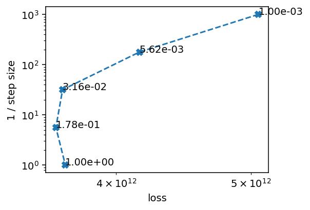
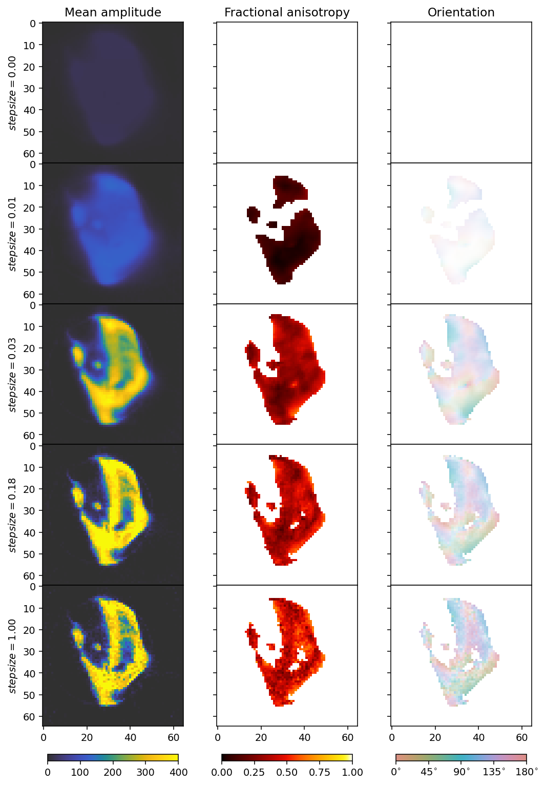
We don’t want steps that are too large or too small, so we go for 0.03 as our step size, which achieves some, but not much reduction in the loss function. We see that a large step size, like 1, already leads to quite a noisy reconstruction.
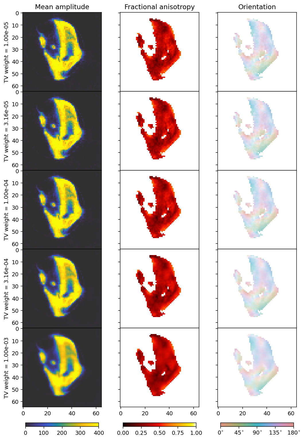
Next, we need to choose a weight for the total variation regularization, and we increase our number of iterations by a factor of 4 for this.
[21]:
tv_weights = np.geomspace(1e-5, 1e-3, 5)
step_size = 0.03 * reference_value
results = []
for t in tv_weights:
    results.append(run_radtt(data_container,
                             step_size=step_size,
                             delta=0.,
                             tv_weight=t * step_size,
                             maxiter=400,
                             update_frequency=50))
Loss: 3.61e+12 Res.norm: 3.61e+12 TV norm: 7.99e+08: 100%|██████████| 400/400 [02:25<00:00,  2.74it/s]
Loss: 3.61e+12 Res.norm: 3.61e+12 TV norm: 7.73e+08: 100%|██████████| 400/400 [02:26<00:00,  2.73it/s]
Loss: 3.62e+12 Res.norm: 3.62e+12 TV norm: 7.06e+08: 100%|██████████| 400/400 [02:27<00:00,  2.72it/s]
Loss: 3.62e+12 Res.norm: 3.62e+12 TV norm: 5.70e+08: 100%|██████████| 400/400 [02:27<00:00,  2.71it/s]
Loss: 3.63e+12 Res.norm: 3.63e+12 TV norm: 4.49e+08: 100%|██████████| 400/400 [02:27<00:00,  2.71it/s]
[22]:
reconstructions = [r['reconstruction'] for r in results]
outputs = [r['basis_set'].get_output(r['reconstruction']) for r in results]
residual_norm = [r['loss_curve'][-1][2] for r in results]
tv_norm = [r['loss_curve'][-1][3] for r in results]
/das/home/carlse_m/p20850/envs/mumott_latest/lib/python3.11/site-packages/mumott/methods/basis_sets/gaussian_kernels.py:490: RuntimeWarning: invalid value encountered in divide
  fractional_anisotropy = fractional_anisotropy / np.sqrt(2*np.sum(eigenvalues**2, axis=-1))
[23]:
fig, axes = plt.subplots(5, 3, figsize=(9.4, 15.6), dpi=140, sharey=True, sharex=True)
for i in range(5):
    ax = axes[i]
    mean, fractional_anisotropy, orientation, alpha = get_2d_images(outputs[i])
    plt.subplots_adjust(wspace=0, hspace=0)
    im0 = ax[0].imshow(mean, **mean_kwargs);
    im1 = ax[1].imshow(fractional_anisotropy, **fractional_anisotropy_kwargs);
    im2 = ax[2].imshow(orientation, alpha=alpha, **orientation_kwargs);
    if i == 0:
        ax[0].set_title('Mean amplitude')
        ax[1].set_title('Fractional anisotropy')
        ax[2].set_title('Orientation')
    ax[0].set_ylabel(r'TV weight = ' + f'{tv_weights[i]:.2e}')
    if i == 4:
        plt.colorbar(im0, ax=axes[:, 0],  **colorbar_kwargs);
        plt.colorbar(im1, ax=axes[:, 1],  **colorbar_kwargs);
        bar = plt.colorbar(im2, ax=axes[:, 2],  **colorbar_kwargs);
        config_cbar(bar)
[24]:
f, ax = plt.subplots(1, 1, figsize=(6, 3), dpi=140)
ax.loglog(residual_norm, tv_norm, '--X')
for x, y, t in zip(residual_norm, tv_norm, tv_weights):
    ax.text(x, y, f'{t:.2e}')
ax.set_ylabel('TV norm')
ax.set_xlabel('Residual norm')
[24]:
Text(0.5, 0, 'Residual norm')
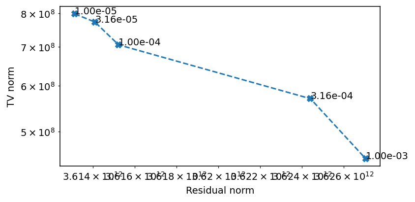
The ideal value seems to be around 1e-4.
Finally, we may want to optimize delta, i.e., the “small value”. As long as we use a large enough number of iterations and momentum in our optimization, and a small enough step size, it is unlikely that changing delta will improve the reconstruction much. However, we can still use this to illustrate what happens when the robust reconstruction becomes more similar to a regular least squares reconstruction.
[25]:
deltas = np.geomspace(1e-3, 1, 5)
tv_weight = 1e-4 * step_size
results = []
for d in deltas:
    results.append(run_radtt(data_container,
                             step_size=step_size,
                             delta=d * reference_value,
                             tv_weight=tv_weight,
                             maxiter=500,
                             update_frequency=100))
Loss: 3.61e+12 Res.norm: 3.61e+12 TV norm: 7.35e+08: 100%|██████████| 500/500 [02:59<00:00,  2.78it/s]
Loss: 3.61e+12 Res.norm: 3.61e+12 TV norm: 7.52e+08: 100%|██████████| 500/500 [03:00<00:00,  2.77it/s]
Loss: 3.59e+12 Res.norm: 3.59e+12 TV norm: 8.51e+08: 100%|██████████| 500/500 [03:01<00:00,  2.76it/s]
Loss: 3.45e+12 Res.norm: 3.45e+12 TV norm: 1.31e+09: 100%|██████████| 500/500 [03:02<00:00,  2.74it/s]
Loss: 3.23e+12 Res.norm: 3.23e+12 TV norm: 2.15e+09: 100%|██████████| 500/500 [03:03<00:00,  2.73it/s]
[26]:
reconstructions = [r['reconstruction'] for r in results]
outputs = [r['basis_set'].get_output(r['reconstruction']) for r in results]
projections = [r['projection'] for r in results]
p_l1 = []
p_l2 = []
for p in projections:
    p_l1.append(np.sum(data_container.weights.ravel() * abs(p.ravel() - data_container.data.ravel())))
    p_l2.append(np.sum(data_container.weights.ravel() * (p.ravel() - data_container.data.ravel()) ** 2))
/das/home/carlse_m/p20850/envs/mumott_latest/lib/python3.11/site-packages/mumott/methods/basis_sets/gaussian_kernels.py:490: RuntimeWarning: invalid value encountered in divide
  fractional_anisotropy = fractional_anisotropy / np.sqrt(2*np.sum(eigenvalues**2, axis=-1))
[27]:
fig, axes = plt.subplots(5, 3, figsize=(9.4, 15.6), dpi=140, sharey=True, sharex=True)
for i in range(5):
    ax = axes[i]
    mean, fractional_anisotropy, orientation, alpha = get_2d_images(outputs[i])
    plt.subplots_adjust(wspace=0, hspace=0)
    im0 = ax[0].imshow(mean, **mean_kwargs);
    im1 = ax[1].imshow(fractional_anisotropy, **fractional_anisotropy_kwargs);
    im2 = ax[2].imshow(orientation, alpha=alpha, **orientation_kwargs);
    if i == 0:
        ax[0].set_title('Mean amplitude')
        ax[1].set_title('Fractional anisotropy')
        ax[2].set_title('Orientation')
    ax[0].set_ylabel(r'delta = ' + f'{deltas[i]:.2e}')
    if i == 4:
        plt.colorbar(im0, ax=axes[:, 0],  **colorbar_kwargs);
        plt.colorbar(im1, ax=axes[:, 1],  **colorbar_kwargs);
        bar = plt.colorbar(im2, ax=axes[:, 2],  **colorbar_kwargs);
        config_cbar(bar)
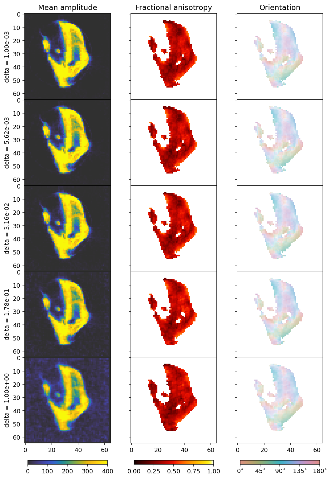
We plot the L1 and L2 norms of the residual to get an understanding of what changes as we modify delta, since this is not entirely easy to infer from the plots, apart from the fact that we see more noise influence with a larger delta.
[28]:
f, ax = plt.subplots(1, 1, figsize=(6, 3), dpi=140)
ax.loglog(p_l1, p_l2, '--X')
for x, y, t in zip(p_l1, p_l2, deltas):
    ax.text(x, y, f'{t:.2e}')
ax.set_ylabel('L2 norm')
ax.set_xlabel('L1 norm')
[28]:
Text(0.5, 0, 'L1 norm')
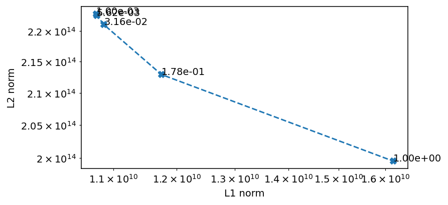
Thus, increasing delta means that we skew the reconstruction toward minimizing the L2 norm, whereas reducing it means that we prefer to minimize the L1 norm. Because the L1 norm is more robust to the influence of noise and outliers, we actually want to keep delta as small as possible, and in this case we would probably be fine Delta at 0.