Optical flow alignment

This tutorial demonstrates the optical flow alignment pipeline in mumott. To this end, we use a publically available experimental data dataset of trabecular bone, for which the alignment has already been done. This allows us to demonstrate the procedure and compare our results to an independent reference.

Since this notebook is relatively sparsely annotated it is advised to start with the tutorial on the phase matching alignment. This will allow you to first obtain a better understanding of the basic challenge and the dataset.

Below we make a copy of the original data and tomographic reconstruction. We then reset the alignment and apply the MITRA pipeline to reconstruct the data. If successful this should allow us to reproduce the quality of the original alignment.

The dataset used in this tutorial is available via Zenodo, and can be downloaded either via a browser or the command line using, e.g., wget or curl:

wget https://zenodo.org/records/10074598/files/trabecular_bone_9.h5

import colorcet
import numpy as np
import matplotlib.pyplot as plt
from matplotlib import gridspec

from mumott.data_handling import DataContainer
from mumott.core.projection_stack import Projection
from mumott.pipelines import run_mitra
from mumott.methods.projectors import SAXSProjector
from mumott.data_handling.utilities import get_absorbances
from mumott.pipelines.utilities import image_processing as imp
from mumott.pipelines import optical_flow_alignment as amo

INFO:Using multiprocessing.cpu_count() to determine the number of availible CPUs.
INFO:Setting the number of threads to 8. If your physical cores are fewer than this number, you may want to use numba.set_num_threads(n), and os.environ["OPENBLAS_NUM_THREADS"] = f"{n}" to set the number of threads to the number of physical cores n.
INFO:Setting numba log level to WARNING.

Loading data

dc = DataContainer('trabecular_bone_9.h5')
geo = dc.geometry
j_offset_reference = geo.j_offsets
k_offset_reference = geo.k_offsets

INFO:Inner axis found in dataset base directory. This will override the default.
INFO:Outer axis found in dataset base directory. This will override the default.
INFO:Rotation matrices were loaded from the input file.
INFO:Sample geometry loaded from file.
INFO:Detector geometry loaded from file.

reconstruction_reference = run_mitra(dc, use_gpu=True, maxiter=20, ftol=None, enforce_non_negativity=True, nestorov_weight=0.6)['result']['x']
absorbances_reference = get_absorbances(dc.diode, normalize_per_projection=True)['absorbances']
sinogram_reference = np.moveaxis(np.squeeze(absorbances_reference), 0, -1)

100%|██████████████████████████████████████████████████████████████████████████████████| 20/20 [00:05<00:00,  3.83it/s]

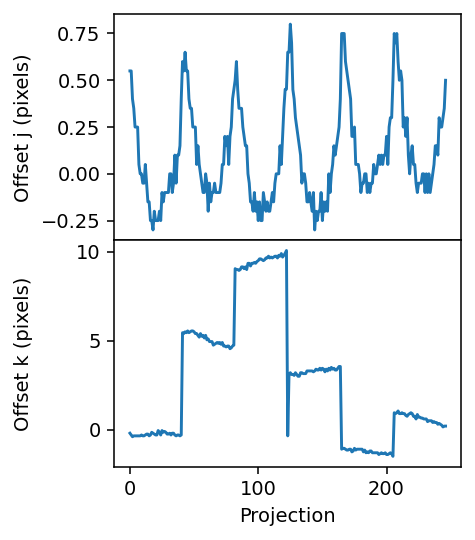
Checking reference alignment

fig, axes = plt.subplots(figsize=(3.2, 4.2), sharex=True, nrows=2, dpi=140)

axes[0].plot(geo.j_offsets)
axes[1].plot(geo.k_offsets)

axes[1].set_xlabel('Projection')
axes[0].set_ylabel('Offset j (pixels)')
axes[1].set_ylabel('Offset k (pixels)')

plt.subplots_adjust(hspace=0)
fig.align_ylabels()

geo.j_offsets = np.zeros(len(geo), dtype=float)
geo.k_offsets = np.zeros(len(geo), dtype=float)
absorbances = get_absorbances(dc.diode, normalize_per_projection=True)['absorbances']

sinogram_0 = np.moveaxis(np.squeeze(absorbances), 0, -1)
diodes_0 = np.moveaxis(np.squeeze(dc.diode), 0, -1)
reconstruction_0 = run_mitra(dc, use_gpu=True, maxiter=20, ftol=None, enforce_non_negativity=True, nestorov_weight=0.6)['result']['x']

100%|██████████████████████████████████████████████████████████████████████████████████| 20/20 [00:04<00:00,  4.34it/s]

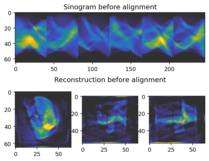
Checking unaligned data

We plot the unaligned data - the sinogram, as well as a virtual slice along each axis.

main_rotation_axis, _ = amo.get_alignment_geometry(dc)
slice_index = sinogram_0.shape[main_rotation_axis] // 2
fig = plt.figure(figsize=(6, 4.8), dpi=140)
gs = gridspec.GridSpec(2, 3)
tomo_kwargs = dict(vmin=0, vmax=0.05, cmap='cet_gouldian')
axes = []
axes.append(fig.add_subplot(gs[0, :]))
for i in range(3):
    axes.append(fig.add_subplot(gs[1, i]))
axes.append(fig.add_subplot(gs[1, :]))
axes[-1].axis('off')

axes[0].imshow(sinogram_0.take(slice_index, axis=main_rotation_axis), cmap='cet_gouldian')
axes[0].set_title("Sinogram before alignment")
axes[1].imshow(reconstruction_0[reconstruction_0.shape[0] // 2, :, :], **tomo_kwargs)
axes[2].imshow(reconstruction_0[:, reconstruction_0.shape[1] // 2, :], **tomo_kwargs)
axes[-1].set_title('Reconstruction before alignment')
axes[3].imshow(reconstruction_0[:, :, reconstruction_0.shape[2] // 2], **tomo_kwargs)

<matplotlib.image.AxesImage at 0x21ca7ad42e0>

Pre-alignment

We compute an initial, crude alignment using the line vertical alignment function.

initial_shift = amo.line_vertical_alignment(dc)
j_offsets, k_offsets = amo.shifts_to_geometry(dc, initial_shift)
geo.j_offsets = j_offsets
geo.k_offsets = k_offsets
j_offset_init = geo.j_offsets
k_offset_init = geo.k_offsets
reconstruction_init = run_mitra(dc, use_gpu=True, maxiter=20, ftol=None, enforce_non_negativity=True, nestorov_weight=0.6)['result']['x']

(65, 55, 247)
100%|██████████████████████████████████████████████████████████████████████████████████| 20/20 [00:04<00:00,  4.46it/s]

fig = plt.figure(dpi=140)
gs = gridspec.GridSpec(2, 3)
tomo_kwargs = dict(vmin=0, vmax=0.05, cmap='cet_gouldian')
axes = []
for i in range(3):
    axes.append(fig.add_subplot(gs[1, i]))
axes.append(fig.add_subplot(gs[1, :]))
axes[-1].axis('off')

axes[0].imshow(reconstruction_init[reconstruction_init.shape[0] // 2, :, :], **tomo_kwargs)
axes[1].imshow(reconstruction_init[:, reconstruction_init.shape[1] // 2, :], **tomo_kwargs)
axes[-1].set_title('Reconstruction after first alignment')
axes[2].imshow(reconstruction_init[:, :, reconstruction_init.shape[2] // 2], **tomo_kwargs)

<matplotlib.image.AxesImage at 0x21ca7295630>

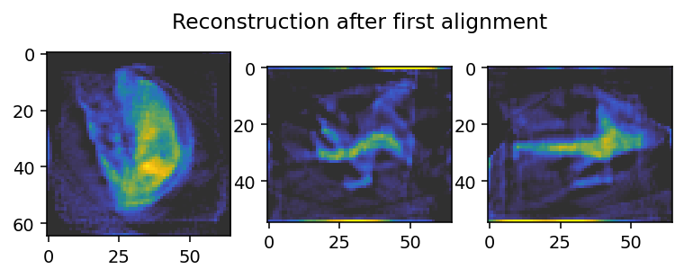
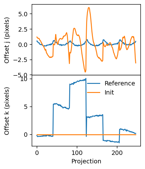
This initial alignment only applies in the j direction.

fig, axes = plt.subplots(figsize=(3.2, 4.2), sharex=True, nrows=2, dpi=140)

axes[0].plot(j_offset_reference)
axes[1].plot(k_offset_reference)
axes[0].plot(geo.j_offsets)
axes[1].plot(geo.k_offsets)
axes[1].legend(['Reference', 'Init'], frameon=False)

axes[1].set_xlabel('Projection')
axes[0].set_ylabel('Offset j (pixels)')
axes[1].set_ylabel('Offset k (pixels)')

plt.subplots_adjust(hspace=0)
fig.align_ylabels()

Step 1: Approximate alignment

For the first alignment step, we use the line_vertical_alignment function to generate an initial approximate alignment. We use only a few iterations for the reconstruction pipeline, and we align both in the horizontal and vertical directions (horizontal is orthogonal to the main rotation axis, vertical is parallel to it). We also center the reconstruction in order to eliminate one degree of freedom.

In addition we apply a smoothing kernel with a standard deviation of 2 pixels.

geo.j_offsets = np.zeros(len(geo), dtype=float)
geo.k_offsets = np.zeros(len(geo), dtype=float)
optimizer_kwargs =  dict(nestorov_weight=0.6, no_tqdm=True)
alignment_param = dict(
    optimal_shift=initial_shift,
    use_gpu=True,
    rec_iteration=5,
    stop_max_iteration=15,
    align_horizontal=True,
    align_vertical=True,
    center_reconstruction=True,
    smooth_data=True,
    sigma_smooth=2.,
    optimizer_kwargs=optimizer_kwargs,
)

# aligning
shifts_1, sinogram_1, _ = amo.run_optical_flow_alignment(dc, **alignment_param)

Alignment iterations: 100%|████████████████████████████████████████████████████████████| 15/15 [02:35<00:00, 10.36s/it]

Checking the alignment

We need to compute the shifts in jk-space in order to check the alignment. We do this using the shifts_to_geometry function.

j_offsets, k_offsets = amo.shifts_to_geometry(dc, shifts_1)
geo.j_offsets = j_offsets
geo.k_offsets = k_offsets
j_offset_1 = geo.j_offsets
k_offset_1 = geo.k_offsets
reconstruction_1 = run_mitra(dc, use_gpu=True, maxiter=20, ftol=None, enforce_non_negativity=True, nestorov_weight=0.6)['result']['x']

100%|██████████████████████████████████████████████████████████████████████████████████| 20/20 [00:04<00:00,  4.57it/s]

fig = plt.figure(figsize=(6, 4.8), dpi=140)
gs = gridspec.GridSpec(2, 3)
tomo_kwargs = dict(vmin=0, vmax=0.05, cmap='cet_gouldian')
axes = []
axes.append(fig.add_subplot(gs[0, :]))
for i in range(3):
    axes.append(fig.add_subplot(gs[1, i]))
axes.append(fig.add_subplot(gs[1, :]))
axes[-1].axis('off')

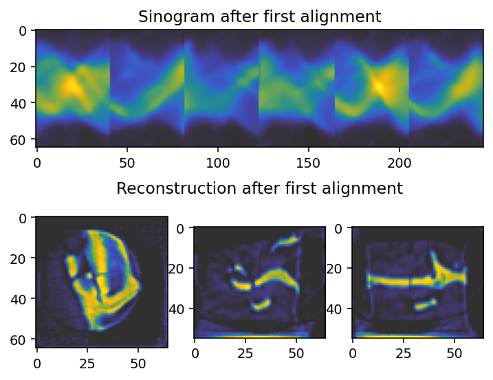
axes[0].imshow(sinogram_1.take(slice_index, axis=main_rotation_axis), cmap='cet_gouldian')
axes[0].set_title("Sinogram after first alignment")
axes[1].imshow(reconstruction_1[reconstruction_1.shape[0] // 2, :, :], **tomo_kwargs)
axes[2].imshow(reconstruction_1[:, reconstruction_1.shape[1] // 2, :], **tomo_kwargs)
axes[-1].set_title('Reconstruction after first alignment')
axes[3].imshow(reconstruction_1[:, :, reconstruction_1.shape[2] // 2], **tomo_kwargs)

<matplotlib.image.AxesImage at 0x21cb11e3f70>

fig, axes = plt.subplots(figsize=(3.2, 4.2), sharex=True, nrows=2, dpi=140)

axes[0].plot(j_offset_reference)
axes[1].plot(k_offset_reference)
axes[0].plot(j_offset_init)
axes[1].plot(k_offset_init)
axes[0].plot(geo.j_offsets)
axes[1].plot(geo.k_offsets)
axes[1].legend(['Reference', 'Init', 'First'], frameon=False)

axes[1].set_xlabel('Projection')
axes[0].set_ylabel('Offset j (pixels)')
axes[1].set_ylabel('Offset k (pixels)')

plt.subplots_adjust(hspace=0)
fig.align_ylabels()

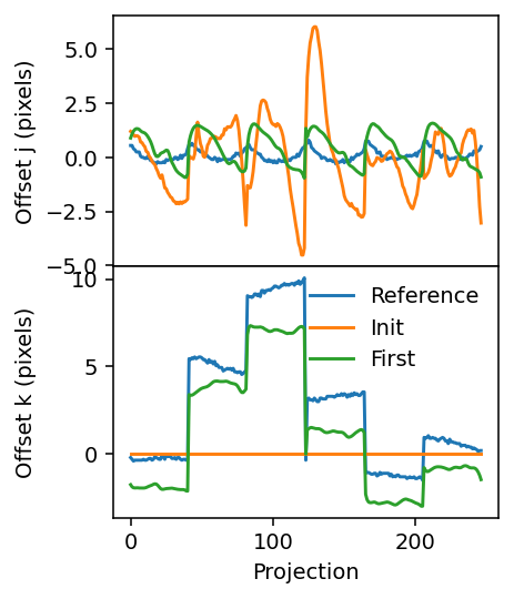
The alignment looks much more similar to the reference alignment now, suggesting that only slight adjustments are needed before a fully satisfactory result is obtained.

Step 2: Refinement

In the second alignment step we increase the number of reconstruction iterations and reduce the number of alignment iterations to align details more precisely. We turn off the centering to avoid perturbing the detailed alignment.

In addition we reduce the standard deviation of the smoothing kernel to one pixel.

geo.j_offsets = np.zeros(len(geo), dtype=float)
geo.k_offsets = np.zeros(len(geo), dtype=float)
alignment_param = dict(
    optimal_shift=shifts_1,
    use_gpu=True,
    rec_iteration=40,
    stop_max_iteration=5,
    align_horizontal=True,
    align_vertical=True,
    center_reconstruction=False,
    smooth_data=True,
    sigma_smooth=1.,
    optimizer_kwargs=optimizer_kwargs,
)

shifts_2, sinogram_2, _ = amo.run_optical_flow_alignment(dc, **alignment_param)

Alignment iterations: 100%|██████████████████████████████████████████████████████████████| 5/5 [01:28<00:00, 17.79s/it]

j_offsets, k_offsets = amo.shifts_to_geometry(dc, shifts_2)
geo.j_offsets = j_offsets
geo.k_offsets = k_offsets
reconstruction_2 = run_mitra(dc, use_gpu=True, maxiter=20, ftol=None, enforce_non_negativity=True, nestorov_weight=0.6)['result']['x']

100%|██████████████████████████████████████████████████████████████████████████████████| 20/20 [00:04<00:00,  4.92it/s]

Checking second alignemnt

fig = plt.figure(figsize=(6, 4.8), dpi=140)
gs = gridspec.GridSpec(2, 3)
tomo_kwargs = dict(vmin=0, vmax=0.05, cmap='cet_gouldian')
axes = []
axes.append(fig.add_subplot(gs[0, :]))
for i in range(3):
    axes.append(fig.add_subplot(gs[1, i]))
axes.append(fig.add_subplot(gs[1, :]))
axes[-1].axis('off')

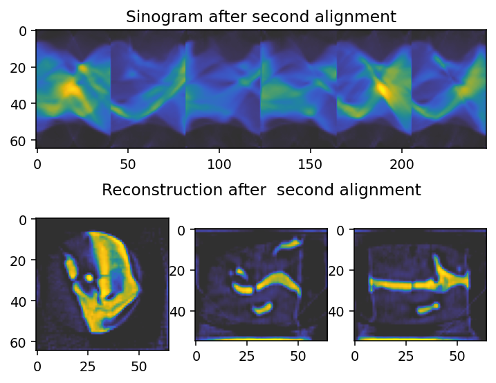
axes[0].imshow(sinogram_2.take(slice_index, axis=main_rotation_axis), cmap='cet_gouldian')
axes[0].set_title("Sinogram after second alignment")
axes[1].imshow(reconstruction_2[reconstruction_2.shape[0] // 2, :, :], **tomo_kwargs)
axes[2].imshow(reconstruction_2[:, reconstruction_2.shape[1] // 2, :], **tomo_kwargs)
axes[-1].set_title('Reconstruction after  second alignment')
axes[3].imshow(reconstruction_2[:, :, reconstruction_2.shape[2] // 2], **tomo_kwargs)

<matplotlib.image.AxesImage at 0x21cbe6062c0>

Final comparison

fig = plt.figure(figsize=(7, 8) , dpi=140)
gs = gridspec.GridSpec(12, 3)
tomo_kwargs = dict(vmin=0, vmax=0.05, cmap='cet_gouldian')
axes = []
ghost_axes = []
for i in range(3):
    for j in range(3):
        axes.append(fig.add_subplot(gs[4 * i:4 * i + 3, j]))
    ghost_axes.append(fig.add_subplot(gs[i + 3 * i, :]))
    ghost_axes[-1].axis('off')

axes = np.array(axes).reshape(3, 3)

axes[2, 0].imshow(reconstruction_0[reconstruction_0.shape[0] // 2, :, :], **tomo_kwargs)
axes[2, 1].imshow(reconstruction_0[:, reconstruction_0.shape[1] // 2, :], **tomo_kwargs)
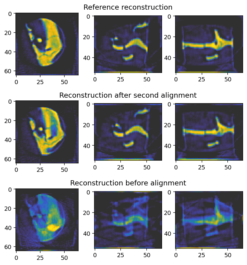
ghost_axes[2].set_title('Reconstruction before alignment')
axes[2, 2].imshow(reconstruction_0[:, :, reconstruction_0.shape[2] // 2], **tomo_kwargs)


axes[1, 0].imshow(reconstruction_2[reconstruction_2.shape[0] // 2, :, :], **tomo_kwargs)
axes[1, 1].imshow(reconstruction_2[:, reconstruction_2.shape[1] // 2, :], **tomo_kwargs)
ghost_axes[1].set_title('Reconstruction after second alignment')
axes[1, 2].imshow(reconstruction_2[:, :, reconstruction_2.shape[2] // 2], **tomo_kwargs)


axes[0, 0].imshow(reconstruction_reference[reconstruction_reference.shape[0] // 2, :, :], **tomo_kwargs)
axes[0, 1].imshow(reconstruction_reference[:, reconstruction_reference.shape[1] // 2, :], **tomo_kwargs)
ghost_axes[0].set_title('Reference reconstruction')
axes[0, 2].imshow(reconstruction_reference[:, :, reconstruction_reference.shape[2] // 2], **tomo_kwargs)

<matplotlib.image.AxesImage at 0x21cbd9d2c20>

Checking final alignment shifts

fig, axes = plt.subplots(figsize=(3.2, 4.2), sharex=True, nrows=2, dpi=140)

axes[0].plot(j_offset_reference)
axes[1].plot(k_offset_reference)
axes[0].plot(j_offset_init)
axes[1].plot(k_offset_init)
axes[0].plot(j_offset_1)
axes[1].plot(k_offset_1)
axes[0].plot(geo.j_offsets)
axes[1].plot(geo.k_offsets)
axes[1].legend(['Reference', 'Init', 'First', 'Second'], frameon=False)

axes[1].set_xlabel('Projection')
axes[0].set_ylabel('Offset j (pixels)')
axes[1].set_ylabel('Offset k (pixels)')

plt.subplots_adjust(hspace=0)
fig.align_ylabels()

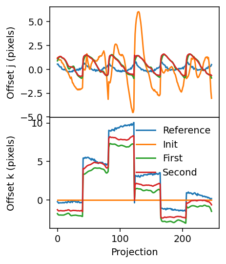
The final shifts are similar but not identical to the reference shifts. They are somewhat offset, which can also be seen in the reference reconstruction.