Reconstruction using pipelines
This tutorial demonstrates the pipelines for simultaneous iterative reconstruction technique (SIRT), the modular iterative tomographic reconstruction algorithm (MITRA), as well as discrete directions (DD), and how they can be used to get started with a reconstruction quickly.
The dataset of trabecular bone used in this tutorial is available via Zenodo, and can be downloaded either via a browser or the command line using, e.g., wget or curl,
wget https://zenodo.org/records/10074598/files/trabecular_bone_9.h5
[1]:
import warnings
from mumott.data_handling import DataContainer
from mumott.pipelines import run_sirt, run_mitra, run_discrete_directions
from mumott.methods.utilities.grids_on_the_sphere import football
from mumott.methods.basis_sets import NearestNeighbor, GaussianKernels
from mumott.optimization.regularizers import HuberNorm, TotalVariation
import matplotlib.pyplot as plt
import colorcet
import logging
import numpy as np
data_container = DataContainer('trabecular_bone_9.h5')
INFO:Setting the number of threads to 4. If your physical cores are fewer than this number, you may want to use numba.set_num_threads(n), and os.environ["OPENBLAS_NUM_THREADS"] = f"{n}" to set the number of threads to the number of physical cores n.
INFO:Setting numba log level to WARNING.
INFO:Inner axis found in dataset base directory. This will override the default.
INFO:Outer axis found in dataset base directory. This will override the default.
INFO:Rotation matrices were loaded from the input file.
INFO:Sample geometry loaded from file.
INFO:Detector geometry loaded from file.
SIRT – simultaneous iterative reconstruction tomography
One of the most straightforward ways to obtain a good reconstruction of transmission data is by using SIRT, which is essentially a preconditioned least-squares formulation of tomography. Because of this preconditioning, the system can be relatively easily solved using gradient descent, and only requires a single parameter, the number of iterations, to be adjusted.
For illustration, in the following cell we run a SIRT reconstruction three times but using a different number of iterations.
[2]:
%%time
logger = logging.getLogger('mumott.optimization.optimizers.gradient_descent')
logger.setLevel(logging.WARNING)

result_1 = run_sirt(data_container,
                    use_gpu=True,
                    maxiter=10)['result']['x']
result_2 = run_sirt(data_container,
                    use_gpu=True,
                    maxiter=100)['result']['x']
result_3 = run_sirt(data_container,
                    use_gpu=True,
                    maxiter=500)['result']['x']
100%|██████████| 10/10 [00:00<00:00, 11.16it/s]
100%|██████████| 100/100 [00:08<00:00, 11.39it/s]
100%|██████████| 500/500 [00:43<00:00, 11.37it/s]
CPU times: user 44.1 s, sys: 13.1 s, total: 57.2 s
Wall time: 57.7 s
[3]:
imshow_kwargs=dict(vmin=0, vmax=0.05, cmap='cet_gouldian')
fig, ax = plt.subplots(1, 3, figsize=(11.6, 3.2), dpi=140, sharey=True)
plt.subplots_adjust(wspace=0)
im = ax[0].imshow(result_1[28, ..., 0], **imshow_kwargs);
im = ax[1].imshow(result_2[28, ..., 0], **imshow_kwargs);
im = ax[2].imshow(result_3[28, ..., 0], **imshow_kwargs);
ax[0].set_title('10 iterations')
ax[1].set_title('100 iterations')
ax[2].set_title('500 iterations')
plt.colorbar(im, ax=ax);
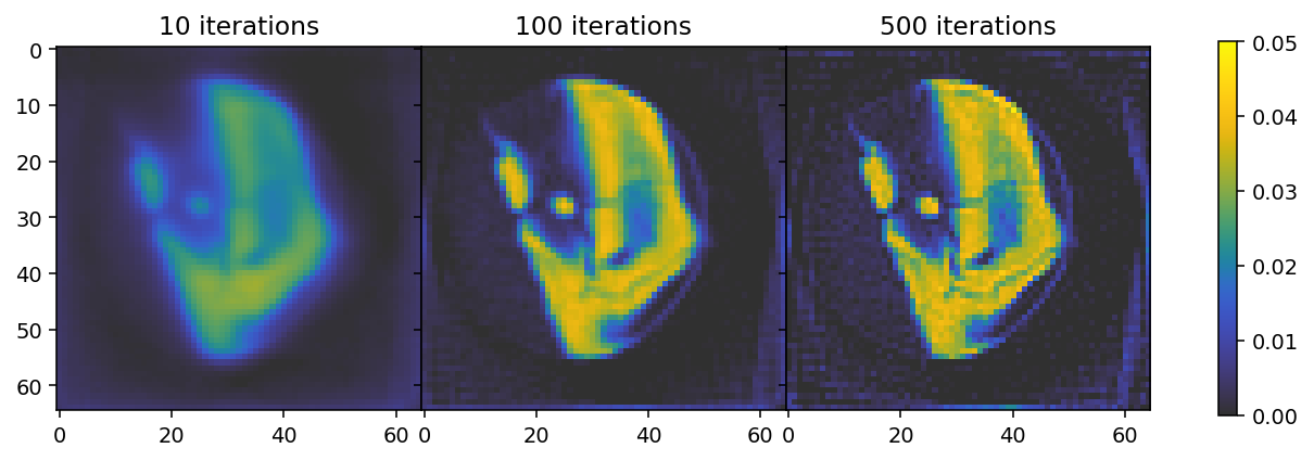
The results show that 10 iterations are insufficient to reach convergence, where the result after 500 iterations indicates overfitting. We can thus conclude that the optimal number of iterations is somewhere between 100 and 500.
MITRA - modular iterative tomographic reconstruction algorithm
While SIRT is easy to get started with and can be straightforwardly extended to tensor-tomography using DD, better reconstructions can be obtained by using regularization, available with MITRA. By default, MITRA also uses a Nestorov gradient in its descent optimization, which greatly improves the rate of convergence. It also uses the same preconditioner as SIRT.
Scalar reconstruction
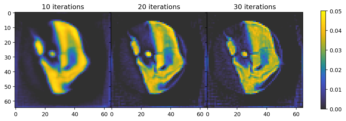
In the following cell we first run the “standard” MITRA pipeline (without regularizers) for three different numbers of iterations. The results illustrate the faster convergence enabled by the Nestorov optimizer used here. By default (use_absorbances=True) the reconstruction is run using the absorbance data, corresponding to the reconstructiong of a scalar field.
[4]:
%%time
result_1 = run_mitra(data_container,
                     use_gpu=True,
                     maxiter=10)['result']['x']
result_2 = run_mitra(data_container,
                     use_gpu=True,
                     maxiter=20)['result']['x']
result_3 = run_mitra(data_container,
                     use_gpu=True,
                     maxiter=30)['result']['x']
100%|██████████| 10/10 [00:00<00:00, 11.35it/s]
100%|██████████| 20/20 [00:01<00:00, 11.39it/s]
100%|██████████| 30/30 [00:02<00:00, 11.36it/s]
CPU times: user 4.85 s, sys: 1.47 s, total: 6.33 s
Wall time: 6.35 s
[5]:
fig, ax = plt.subplots(1, 3, figsize=(11.6, 3.2), dpi=140, sharey=True)
plt.subplots_adjust(wspace=0)
im = ax[0].imshow(result_1[28, ..., 0], **imshow_kwargs);
im = ax[1].imshow(result_2[28, ..., 0], **imshow_kwargs);
im = ax[2].imshow(result_3[28, ..., 0], **imshow_kwargs);
ax[0].set_title('10 iterations')
ax[1].set_title('20 iterations')
ax[2].set_title('30 iterations')
plt.colorbar(im, ax=ax);
Scalar reconstruction with regularization
This is only the start. We can also attach regularizers to MITRA, further improving the reconstruction. We will illustrate this with the HuberNorm and TotalVariation regularizers.
The HuberNorm regularizer suppresses noise while converging more easily than a traditional \(L_1\) norm. The latter is achieved by switching from the \(L_1\) to the \(L_2\) norm for residuals below a threshold value that is set by the delta parameter.
The TotalVariation regularizer adds smoothness while preserving edges, and like the HuberNorm, is spliced with a more easily converging function below a threshold set by its respective delta parameter.
Here, we set the delta parameter to 1e-2, representing a typical “small” value in the reconstruction.
[6]:
%%time
def get_regularizers(alpha, beta):
    return [dict(name='hn', regularizer=HuberNorm(delta=1e-2), regularization_weight=alpha),
            dict(name='tv', regularizer=TotalVariation(delta=1e-2), regularization_weight=beta)]
alpha_values = np.geomspace(2e-3, 2e-5, 3)
beta_values = np.geomspace(1e-4, 1e-6, 3)
result = []
values = []
for alpha in alpha_values:
    for beta in beta_values:
        result.append(run_mitra(data_container,
                                use_gpu=True,
                                maxiter=30,
                                Regularizers=get_regularizers(alpha, beta))['result']['x'])
        values.append((alpha, beta))
100%|██████████| 30/30 [00:02<00:00, 10.57it/s]
100%|██████████| 30/30 [00:02<00:00, 10.57it/s]
100%|██████████| 30/30 [00:02<00:00, 10.54it/s]
100%|██████████| 30/30 [00:02<00:00, 10.54it/s]
100%|██████████| 30/30 [00:02<00:00, 10.54it/s]
100%|██████████| 30/30 [00:02<00:00, 10.55it/s]
100%|██████████| 30/30 [00:02<00:00, 10.50it/s]
100%|██████████| 30/30 [00:02<00:00, 10.52it/s]
100%|██████████| 30/30 [00:02<00:00, 10.50it/s]
CPU times: user 22.5 s, sys: 6.32 s, total: 28.8 s
Wall time: 29 s
[7]:
fig, ax = plt.subplots(3, 3, figsize=(11., 9.4), dpi=140, sharey='row', sharex='col')
plt.subplots_adjust(wspace=0.00, hspace=0.)
for i in range(3):
    ax[i, 0].set_ylabel(r'$\alpha = {:0.0e}$'.format(values[i*3][0]))
    for j in range(3):
        im = ax[i, j].imshow(result[i*3 + j][28, ..., 0], **imshow_kwargs);
        ax[2, j].set_xlabel(r'$\beta = {:0.0e}$'.format(values[i*3 + j][1]))
plt.colorbar(im, ax=ax, shrink=0.5, pad=0.0);
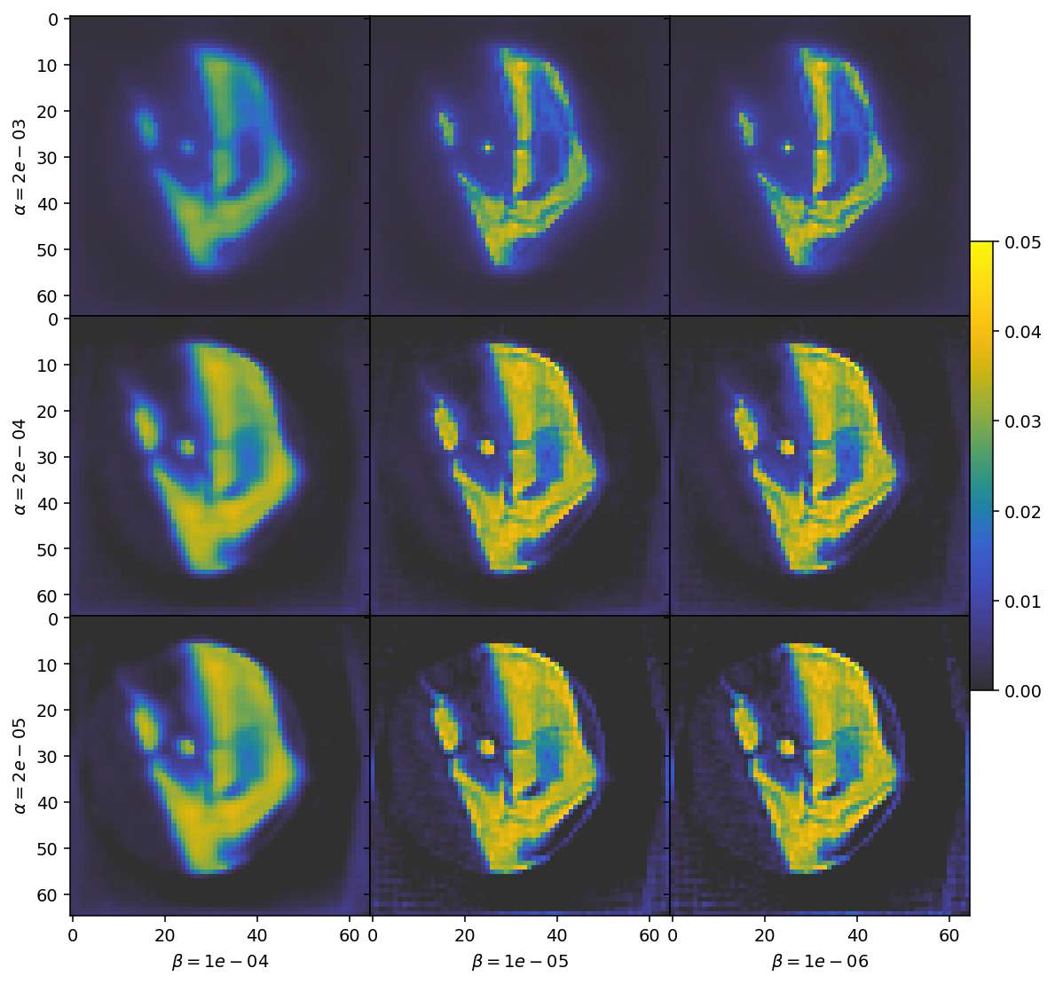
The top row has large parts of the expected reconstruction blanked out due to over-regularization. Conversely the bottom row has barely any noise suppression at all. Similarly, the highly regularized cases to the left become blurry, while the under-regularized cases to the right become grainy.
We are thus looking for a choice in the middle of these extremes. Based on this visual inspection, we should select values of \(\alpha = 2e-4\) and \(\beta = 1e-5\) for our regularization parameters.
Application to tensor tomography
MITRA is not limited to scalar reconstruction but be applied to tensor tomography as well. By default it will use GaussianKernels to represent functions on the sphere, and apply tensor SIRT weights.
For demonstration, we run the MITRA pipeline using the “full” data from the data container (i.e., we do not limit us to the absorbances).
[8]:
%%time
results = run_mitra(data_container,
                    use_gpu=True,
                    maxiter=30,
                    use_absorbances=False)

reconstruction = results['result']['x']
output = results['basis_set'].get_output(reconstruction)
100%|██████████| 30/30 [00:29<00:00,  1.03it/s]
CPU times: user 49.6 s, sys: 10.9 s, total: 1min
Wall time: 35.2 s
/das/home/carlse_m/p20850/envs/mumott_latest/lib/python3.11/site-packages/mumott/methods/basis_sets/gaussian_kernels.py:490: RuntimeWarning: invalid value encountered in divide
  fractional_anisotropy = fractional_anisotropy / np.sqrt(2*np.sum(eigenvalues**2, axis=-1))
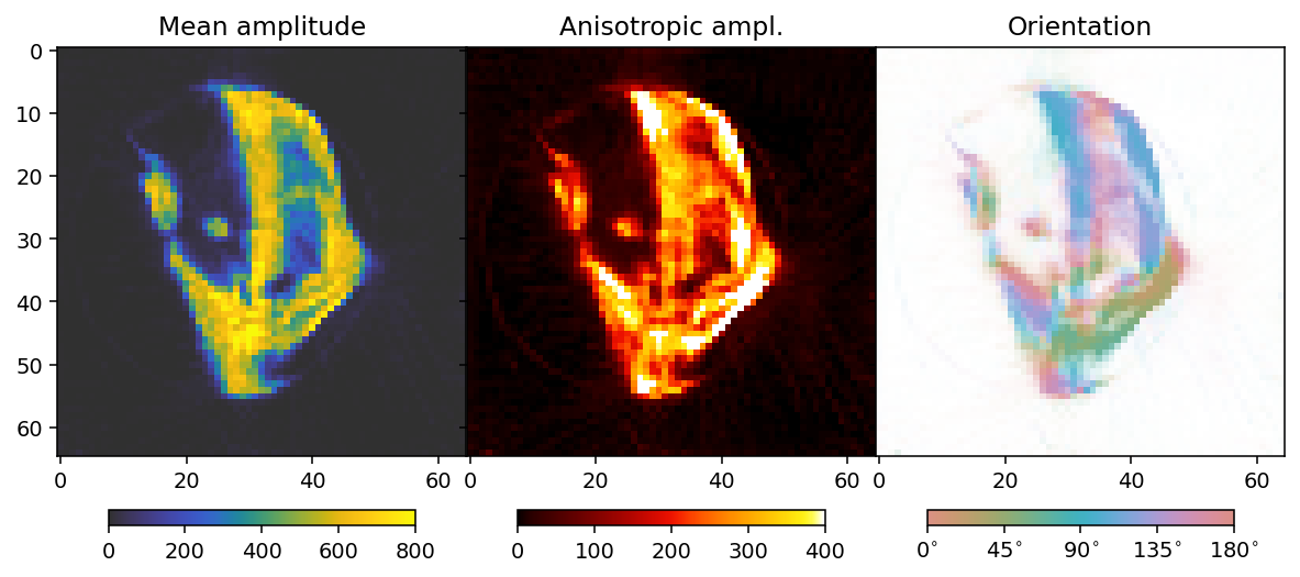
To analyze the results we here define a convenience function that allows us to extract mean, fractional anisotropy, and orientation data in a 2D slice from the reconstruction.
The function defined here uses output.eigenvector_1 which corresponds to the direction with lowest scattering, For equatorial ring type scattering output.eigenvector_1 is apropriate. For polar cap type scattering, output.eigenvector_3.
[9]:
plotted_slice_index = 28
mask_threshold = 100

def get_2d_images(output):

    mean = output.mean_intensity[plotted_slice_index]
    mask = mean > mask_threshold

    fractional_anisotropy = output.fractional_anisotropy[plotted_slice_index]
    fractional_anisotropy[~mask] = 1

    main_eigenvector = output.eigenvector_1[plotted_slice_index]
    orientation = np.arctan2(-main_eigenvector[..., 1],
                             main_eigenvector[..., 2])
    orientation[orientation < 0] += np.pi
    orientation[orientation > np.pi] -= np.pi
    orientation *= 180 / np.pi

    alpha = np.clip(output.fractional_anisotropy[plotted_slice_index], 0, 1)
    alpha[~mask] = 0

    return mean, fractional_anisotropy, orientation, alpha
[10]:
mean, fractional_anisotropy, orientation, alpha = get_2d_images(output)
Next we plot the results.
[11]:
colorbar_kwargs = dict(orientation='horizontal', shrink=0.75, pad=0.1)
mean_kwargs = dict(vmin=0, vmax=400, cmap='cet_gouldian')
fractional_anisotropy_kwargs = dict(vmin=0, vmax=1.0, cmap='cet_fire')
orientation_kwargs = dict(vmin=0, vmax=180, cmap='cet_CET_C10')

def config_cbar(cbar):
    cbar.set_ticks([i for i in np.linspace(0, 180, 5)])
    cbar.set_ticklabels([r'$' + f'{int(v):d}' + r'^{\circ}$' for v in bar.get_ticks()])
[12]:
fig, ax = plt.subplots(1, 3, figsize=(10.3, 4.6), dpi=140, sharey=True)

im0 = ax[0].imshow(mean, **mean_kwargs);
im1 = ax[1].imshow(fractional_anisotropy, **fractional_anisotropy_kwargs);
im2 = ax[2].imshow(orientation, alpha=alpha, **orientation_kwargs);

ax[0].set_title('Mean amplitude')
ax[1].set_title('Fractional anisotropy')
ax[2].set_title('Orientation')

plt.subplots_adjust(wspace=0)

plt.colorbar(im0, ax=ax[0], **colorbar_kwargs)
plt.colorbar(im1, ax=ax[1], **colorbar_kwargs)
bar = plt.colorbar(im2, ax=ax[2], **colorbar_kwargs)
config_cbar(bar)
Tensor reconstruction with regularization
We can regularize our reconstruction in a very similar manner as for the scalar case. To keep the plots clear, we start by only running over beta and thus limit ourselves to the TotalVariation regularizer. We set delta=1 as there is no single optimal value correspoding to a “small” number; one could reasonably set it anywhere between 0.8 and 80. A larger number will make the reconstruction converge more easily, but a smaller number will be more effective for removing noise. As a
general guideline, one thus would like to use the smallest number that for which convergence can be achieved (with reasonable effort).
[13]:
%%time
def get_regularizers(alpha=0, beta=0):
    return [dict(name='hn', regularizer=HuberNorm(delta=1), regularization_weight=alpha),
            dict(name='tv', regularizer=TotalVariation(delta=1), regularization_weight=beta)]
beta_values = np.geomspace(0.5, 5, 3)
result = []
values = []
for beta in beta_values:
    result.append(run_mitra(data_container,
                            use_gpu=True,
                            maxiter=30,
                            use_absorbances=False,
                            Regularizers=get_regularizers(beta=beta)))
    values.append(beta)
100%|██████████| 30/30 [01:01<00:00,  2.04s/it]
100%|██████████| 30/30 [00:58<00:00,  1.96s/it]
100%|██████████| 30/30 [00:56<00:00,  1.90s/it]
CPU times: user 3min 26s, sys: 52.3 s, total: 4min 18s
Wall time: 3min 2s
[15]:
reconstructions = [r['result']['x'] for r in result]
outputs = [r['basis_set'].get_output(r['result']['x']) for r in result]
[16]:
colorbar_kwargs = dict(orientation='horizontal', shrink=0.75, pad=0.033)
fig, axes = plt.subplots(3, 3, figsize=(9.4, 11.6), dpi=140, sharey=True, sharex=True)
for i in range(3):
    ax = axes[i]
    mean, fractional_anisotropy, orientation, alpha = get_2d_images(outputs[i])
    plt.subplots_adjust(wspace=0, hspace=0)
    im0 = ax[0].imshow(mean, **mean_kwargs);
    im1 = ax[1].imshow(fractional_anisotropy, **fractional_anisotropy_kwargs);
    im2 = ax[2].imshow(orientation, alpha=alpha, **orientation_kwargs);
    if i == 0:
        ax[0].set_title('Mean amplitude')
        ax[1].set_title('Fractional anisotropy')
        ax[2].set_title('Orientation')
    ax[0].set_ylabel(r'$\beta = ' + f'{beta_values[i]:.2f}' + r'$')
    if i == 2:
        plt.colorbar(im0, ax=axes[:, 0], **colorbar_kwargs);
        plt.colorbar(im1, ax=axes[:, 1], **colorbar_kwargs);
        bar = plt.colorbar(im2, ax=axes[:, 2], **colorbar_kwargs);
        config_cbar(bar)
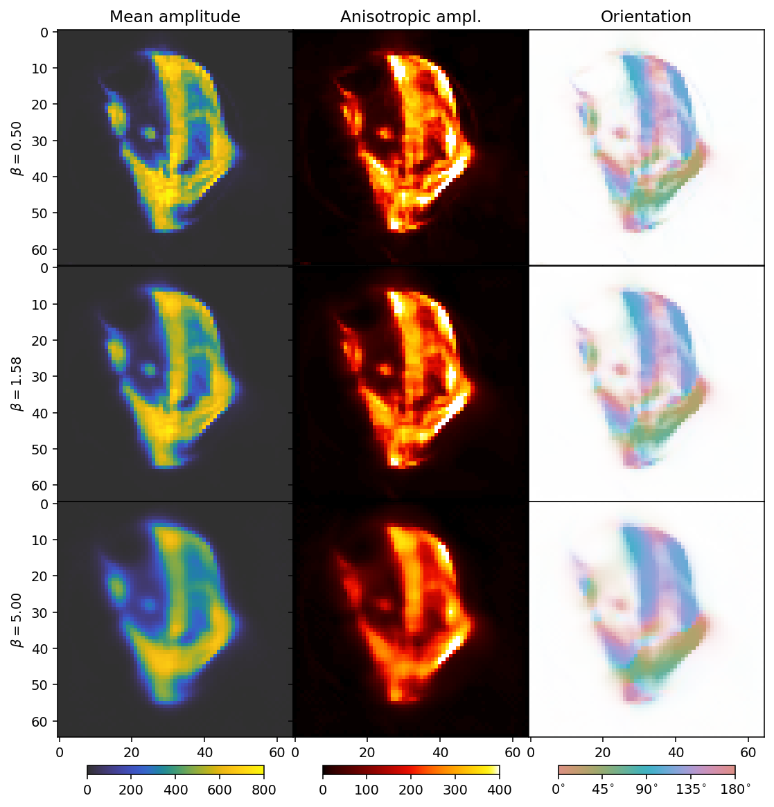
As before with increasing beta, the reconstructions become blurrier. The comparison suggests that a suitable choice for beta should be close to the middle row.
Next we scan different values for alpha (HuberNorm) with beta=2 (TotalVariation).
[17]:
%%time
alpha_values = np.geomspace(1, 40, 3)
result = []
values = []
for alpha in alpha_values:
    result.append(run_mitra(data_container,
                  use_gpu=True,
                  maxiter=30,
                  use_absorbances=False,
                  Regularizers=get_regularizers(alpha=alpha, beta=2.)))
    values.append(alpha)
100%|██████████| 30/30 [00:57<00:00,  1.93s/it]
100%|██████████| 30/30 [00:56<00:00,  1.87s/it]
100%|██████████| 30/30 [00:53<00:00,  1.80s/it]
CPU times: user 3min 15s, sys: 53.9 s, total: 4min 9s
Wall time: 2min 53s
[18]:
reconstructions = [r['result']['x'] for r in result]
outputs = [r['basis_set'].get_output(r['result']['x']) for r in result]
/das/home/carlse_m/p20850/envs/mumott_latest/lib/python3.11/site-packages/mumott/methods/basis_sets/gaussian_kernels.py:490: RuntimeWarning: invalid value encountered in divide
  fractional_anisotropy = fractional_anisotropy / np.sqrt(2*np.sum(eigenvalues**2, axis=-1))
[19]:
fig, axes = plt.subplots(3, 3, figsize=(9.4, 11.6), dpi=140, sharey=True, sharex=True)
for i in range(3):
    ax = axes[i]
    mean, fractional_anisotropy, orientation, alpha = get_2d_images(outputs[i])
    plt.subplots_adjust(wspace=0, hspace=0)
    im0 = ax[0].imshow(mean, **mean_kwargs);
    im1 = ax[1].imshow(fractional_anisotropy, **fractional_anisotropy_kwargs);
    im2 = ax[2].imshow(orientation, alpha=alpha, **orientation_kwargs);
    if i == 0:
        ax[0].set_title('Mean amplitude')
        ax[1].set_title('Fractional anisotropy')
        ax[2].set_title('Orientation')
    ax[0].set_ylabel(r'$\alpha = ' + f'{alpha_values[i]:.2f}' + r'$')
    if i == 2:
        plt.colorbar(im0, ax=axes[:, 0],  **colorbar_kwargs);
        plt.colorbar(im1, ax=axes[:, 1],  **colorbar_kwargs);
        bar = plt.colorbar(im2, ax=axes[:, 2],  **colorbar_kwargs);
        config_cbar(bar)
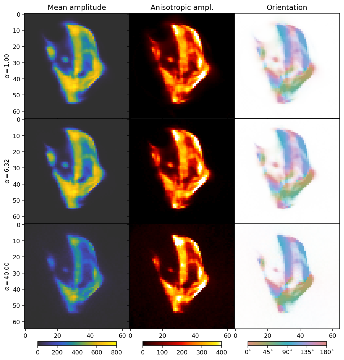
We can now see the effect of the \(L_1\) regularizer. It has a broad dampening effect that first only acts on the background, but eventually becomes strong enough to dampen the entire reconstruction.
The comparison suggests a value for alpha somewhere in the range from 6 (middle row) to 40 (bottom row). Generally, one must start with a broader sweep than we have done in this tutorial, where we already start with good guesses. In practice a regularization parameter typically sweep might span 10 to 15 orders of magnitude.
DD - discrete directions
Rather than regularizing by imposing constraints on the whole solution, we can place the measured reciprocal space map components into bins on the sphere, and reconstruct each bin independently. This is what the DD pipeline does. Each reconstruction is that solved by SIRT. The drawback of this method is that it is not compatible with constraint-based regularization. However, due to the inherent regularization properties of SIRT, smooth reconstructions can be obtained by using a small number
of iterations in the reconstruction.
In the following cells, we run the reconstruction and plot the result. The reconstruction shown uses the same grid as the GaussianKernels of the MITRA pipelines, for easy comparison.
[20]:
%%time
theta, phi = GaussianKernels(grid_scale=5).grid
directions = np.concatenate(((np.sin(theta) * np.cos(phi))[:, None], (np.sin(theta) * np.sin(phi))[:, None], np.cos(theta)[:, None]), axis=1)
result = []
maximum_iterations = [10, 100, 300]
for maxiter in maximum_iterations:
    result.append(run_discrete_directions(data_container, directions, maxiter=maxiter, use_gpu=True))
100%|██████████| 72/72 [01:24<00:00,  1.17s/it]
100%|██████████| 72/72 [00:53<00:00,  1.34it/s]
100%|██████████| 72/72 [02:32<00:00,  2.12s/it]
CPU times: user 4min 38s, sys: 7 s, total: 4min 45s
Wall time: 4min 50s
[21]:
reconstructions = [r['result']['x'] for r in result]
outputs = [r['basis_set'].get_output(r['result']['x']) for r in result]
/das/home/carlse_m/p20850/envs/mumott_latest/lib/python3.11/site-packages/mumott/methods/basis_sets/nearest_neighbor.py:468: RuntimeWarning: invalid value encountered in divide
  fractional_anisotropy = fractional_anisotropy / np.sqrt(2*np.sum(eigenvalues**2, axis=-1))
We calculate a number of scalar quantities from the tensor tomography solution for plotting.
[22]:
mean_kwargs = dict(vmin=0, vmax=800, cmap='cet_gouldian')
colorbar_kwargs = dict(orientation='horizontal', shrink=0.75, pad=0.033)
fig, axes = plt.subplots(3, 3, figsize=(9.4, 11.6), dpi=140, sharey=True, sharex=True)
for i in range(3):
    ax = axes[i]
    mean, fractional_anisotropy, orientation, alpha = get_2d_images(outputs[i])
    plt.subplots_adjust(wspace=0, hspace=0)
    im0 = ax[0].imshow(mean, **mean_kwargs);
    im1 = ax[1].imshow(fractional_anisotropy, **fractional_anisotropy_kwargs);
    im2 = ax[2].imshow(orientation, alpha=alpha, **orientation_kwargs);
    if i == 0:
        ax[0].set_title('Mean amplitude')
        ax[1].set_title('Fractional anisotropy')
        ax[2].set_title('Orientation')
    ax[0].set_ylabel(r'$maxiter = ' + f'{maximum_iterations[i]}' + r'$')
    if i == 2:
        plt.colorbar(im0, ax=axes[:, 0], **colorbar_kwargs);
        plt.colorbar(im1, ax=axes[:, 1], **colorbar_kwargs);
        bar = plt.colorbar(im2, ax=axes[:, 2], **colorbar_kwargs);
        config_cbar(bar)
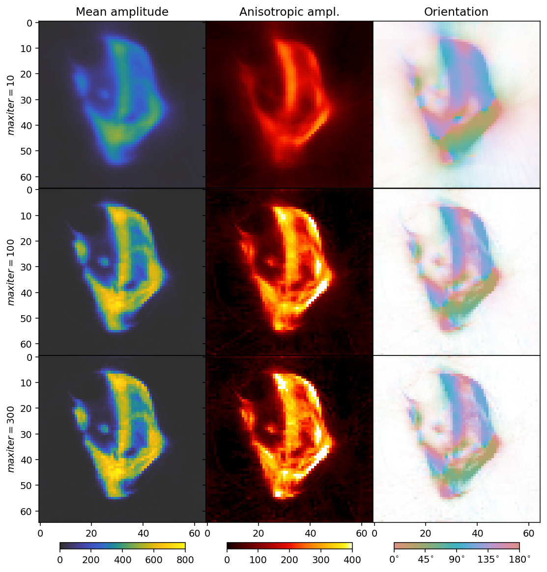
From this reconstruction, we can see that about 100 iterations is a good number, and the quality of the reconstruction as far as can be assessed from the mean, standard deviation, and orientations of this slice, is comparable to that of the regularized GaussianKernels reconstruction.